
 Open access


1. Introduction
The search for organizing principles of visual processing in cortex has proven long and fruitful, demonstrating specific types of organization arising on multiple scales (e.g., magno-cellular / parvo-cellular pathways [1] and ocular dominance columns [2]). One of the more important larger scale organizing principles of visual cortical organization is the visual field map (VFM): neurons whose visual receptive fields lie next to one another in visual space are located next to one another in cortex, forming one complete representation of contralateral visual space [3]. Each VFM subserves a specific computation or set of computations; locating these VFMs allows for the systematic exploration of these computations across visual cortex [4, 5]. It has been suggested that this retinotopic organization of VFMs allows for efficient connectivity between neurons that represent nearby locations in visual space, likely necessary for such processes as lateral inhibition and gain control [6-9]. This chapter will discuss the primary neuroimaging techniques used for measuring human VFMs, our current understanding of the organization of visuospatial representations across human visual cortex, the present state of our knowledge of white matter connectivity among these representations, and how these measurements inform us about the functional divisions of visual cortex in human.
2. Neuroimaging methods for measuring human visual field maps
VFMs are routinely measured in the
In human measurements, the most compelling evidence for visual areas is the VFMs, also commonly called retinotopic maps. In short, a VFM is a visual area with a complete representation of visual space, where neurons that represent adjacent locations on the retina (and visual space) are also adjacent in cortex [12]. Because many computations are required to create our visual experience, our brains have many specialized VFMs which perform one or more of those computations across the entire visual scene (e.g., motion perception happens throughout our visual field, not just in the upper left quadrant). By taking advantage of the knowledge of the retinotopic organization of visual input, multiple cortical VFMs can be measured using fMRI with respect to the two orthogonal dimensions needed to identify a unique location in visual space: eccentricity and polar angle. This chapter will review two of the most powerful fMRI techniques for very detailed measurements of VFM in individual subjects: travelling wave retinotopy (TWR) [10] and population receptive field (pRF) modeling [22].
2.1. The standard paradigm: Travelling wave retinotopy
TWR has been the gold standard for visual field mapping since its development in the mid 1990‘s (Figure 1) [10, 23-26]. This technique uses two types of periodic stimuli that move smoothly across a contiguous region of visual space to measure the orthogonal dimensions of polar angle and eccentricity. One stimulus is designed to elicit each voxel‘s preferred polar angle by presenting a high-contrast, flickering checkerboard stimulus shaped like a wedge that spans the fovea to periphery along a small range of specific polar angles (Figure 2A). The wedge stimulus rotates either clockwise or counterclockwise in discrete even steps around the central fixation point to sequentially activate distinct polar angle representations of visual space. The second stimulus is designed to elicit each fMRI voxel‘s preferred eccentricity by presenting a stimulus shaped like a ring, which expands or contracts in discrete even steps between the central fovea and the periphery (Figure 2B). The measurement of these
These traveling-wave stimuli are typically comprised of a set of high contrast checkerboard patterns that are designed to maximally stimulate primary visual cortex and generally elicit an fMRI signal modulation on the order of 1%–3% (Figures 1-2). This modulation is typically 15–20 standard deviations above the background noise. Stimuli comprised of other shapes (e.g., faces, objects) have also been used in studies interested in measuring the retinotopic organization of higher order visual cortex, but the high contrast checkerboard stimulus has proven to drive even these regions well in many studies[26, 27].

Figure 1.
Visual Field Mapping Time Series Analysis. Each row represents the activity and analysis of a time series of a single 6-cycle scan of one type of experimental stimuli (expanding rings or rotating wedges) for a single voxel. Black dots indicate simulated raw data points of % blood oxygen level-dependent (BOLD) modulation. The red lines indicate the peak activations per cycle for an imaginary set of voxels, which are the measurements used by the traveling wave retinotopy (TWR) analysis. The blue dotted line represents a sinusoidal fit of the simulated data points, which are the measurements used by population receptive field (pRF) modeling. Rows (A) and (B) represent time series of voxels with identical %BOLD modulation, but different peak responses, which indicate different stimulus selectivity (different ‘phases’ of response). For example, (A) might represent a voxel with a preferred eccentricity tuning of 5° eccentric to fixation, whereas (B) might have a preferred tuning of only 2° eccentric to fixation. Rows (A) and (C) represent time series of voxels with identical peak responses, indicating identical stimulus selectivity. However, (C) has much lower %BOLD modulation than (A), which may be due to two primary factors: differences in local vasculature or broader receptive field tuning for (C) than (A).
In each scan, only one stimulus is presented, and all of visual space is cycled through several times with each stimulus (Figure 1). Typically, several scans are then averaged together for each stimulus type to increase the fMRI blood oxygen level-dependent (BOLD) signal to noise ratio. These stimuli create a travelling wave of cortical activity that travels from one end of the VFM to the other along iso-angle or iso–eccentricity lines, giving TWR its name. Thus the time, or phase, of the peak modulation varies smoothly across the cortical surface. This phase defines the most effective stimulus eccentricity (ring) and polar angle (wedge) to activate that region of cortex, giving TWR its description as ‘phase-encoded retinotopy.’ In TWR data, the phase of the response is represented as a color-coded overlay on anatomical data (Figure 2). It is important to note that these types of TWR stimuli are not only excellent for measuring cortical VFMs, but that they only produce activity in regions that are retinotopically-organized.

Figure 2.
TWR Measurements. Traveling wave stimuli typically consist of a set of high contrast checkerboard patterns that move smoothly and periodically through a range of eccentricities (ring) or polar angles (wedge). The inflated cortical surface (inset) is labeled as follows: CC, corpus callosum; POS, parietal-occipital sulcus; CaS, calcarine sulcus. An expanded view of this surface near calcarine sulcus is overlaid with a color map showing the response phase at each location for polar angle (A) and eccentricity experiments (B) (see the colored legend insets). The stimuli covered the central 16° radius of visual space. The solid white lines indicate the boundaries of visual area V1 in the calcarine sulcus. For clarity, the colored visual responses are only overlaid on locations near the calcarine sulcus, and only voxels with a powerful response at a coherence ≥ 0.25 are colored.
The design of TWR presents all eccentricities or polar angles at a given frequency per scan (typically 6-8 cycles per scan), which allows the use of a Fourier analysis. TWR only considers activity that is at this signal frequency, excluding low-frequency physiological noise, among other things. The statistical threshold for cortical activity arising from the TWR stimulus is commonly determined by
2.2. An innovative approach to measure the organization of human visual cortex: Population receptive field modeling
Once it became clear that there were limits to the ability of TWR to deal with VFMs with large RFs, researchers at Stanford University decided to improve VFM measurements by developing a new method that models the pRFs of each voxel within VFMs [22]. This model relies on the logic that, because VFMs are retinotopically organized, the population of RFs in each voxel of a VFM is expected to have similar preferred centers and sizes, allowing their combined pRF to be estimated as a single, two-dimensional Gaussian RF. Despite the fact that there is some variability in the neural RFs of each voxel in terms of their preferred centers and sizes, termed RF scatter, the pRF provides a good, if somewhat slightly larger, estimate of the individual neural RFs in the voxel. The advantages of the method are generally stated in comparison to TWR, as the field standard for measuring VFMs. The pRF method provides an accurate estimate of not only the preferred center for each voxel’s pRF (as in TWR), but also its size (Figures 3, 4). In addition, the method does not require two distinct stimuli to measure orthogonal dimensions of visual space as in TWR, cutting down on the total number of scans necessary per subject.

Figure 3.
Measurements of an Individual Voxel. (A) A typical voxel recorded from a popular 3 Tesla MRI scanner is on the order of 1 mm3, though often slightly larger (2-3 mm3). (B) Within each typical voxel, there are on the order of ~1 million neurons, depending on the size of the voxel. For voxels in retinotopic visual cortex, the neurons each have similarly located spatial receptive fields (black outlines) with preferred centers (black dots). (C) Traveling wave retinotopy (TWR) takes advantage of the fact that nearby neurons in retinotopic cortex have similar preferred centers in order to estimate a population preferred center for the population of neurons in a given voxel. (D) Population receptive field (pRF) modeling takes advantage of the fact that nearby neurons in retinotopic cortex have similar receptive fields in order to estimate not only a preferred center, but also a pRF for the population of neurons in a given voxel.
To accomplish this, the pRF model first creates a very large database of possible pRF sizes and centers that cover the field of view of the stimulus (Figure 4). Then, the model convolves each of the pRF possibilities with a standard hemodynamic response function (HRF). Finally, the model uses a least-squares fitting method to iteratively test each of the pRF possibilities for each voxel independently against the actual data collected. Whichever pRF best fits the data is then assigned as the pRF for that voxel. Only voxels that contain activity above a chosen threshold of variance explained as determined by the model are included for further analysis.
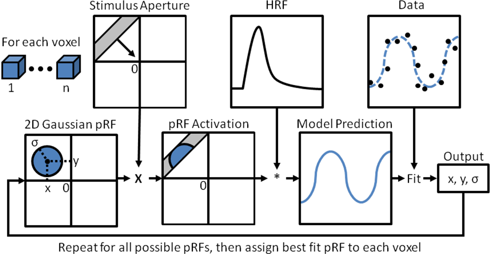
Figure 4.
Population Receptive Field Modeling. The parameter estimation procedure for the population receptive field (pRF) model is shown as a flow chart. The example stimulus aperture is a moving bar stimulus. Adapted from
Although it is technically possible to use any stimulus that systematically traverses the entire field of view, typically the stimulus takes one of two forms. First is a slightly modified version of the TWR stimuli, in which neutral gray blank periods are inserted at an off-frequency from the stimulus frequency (i.e., 4 instead of 6-8 cycles/scan, so they are separable in the Fourier analysis). The second and increasingly common stimulus is a high-contrast flickering checkerboard bar stimulus that steps across the field of view in the 8 cardinal directions, again with several interspersed neutral gray blank periods. The neutral gray blank periods allow for an estimation of a voxel’s response to any visual stimulus versus just the preferred visual stimulus, which is crucial for the accurate measurement of pRF sizes. In theory, one could also tile visual space using any stimulus of interest, if the aforementioned stimuli do not drive the area well. Since the checkerboard stimuli were designed to drive activity in early visual cortex, it is possible other stimuli containing more complex may perform better in higher-order VFMs.
The pRF method has the additional benefit of measuring other neuronal population properties, such as receptive field size and laterality. These pRF measurements can demonstrate differences in the internal receptive field structures between, for example, a hemifield map in primary visual cortex (V1) and a hemifield map in lateral cortex (e.g., LO-1; [28]). With the traveling wave method, both maps look very similar, as only the peak time series responses are measured. However, the underlying properties of the neuronal populations within these two maps are actually quite different, with finely tuned neurons in V1 and more broadly tuned neurons in lateral cortex. The models of the underlying neuronal properties from the pRF method can measure these receptive field differences, as well as the amount of input from ipsi- and contralateral visual fields (e.g., [29]). The human pRF size estimates for V1/V2/V3 reported by Dumoulin and Wandell [22] agree well with electrophysiological receptive field measurements at a range of eccentricities in corresponding locations within primate VFMs.
These pRF methods have successfully been used by a small group of labs to (1) investigate the normal organization of human visual cortex (e.g., [12, 29, 30]), (2) measure developmental plasticity in achiasmatic and sight recovery patients [31, 32], and (3) examine cortical reorganization in aged-related macular degeneration [33]. Because pRF Modeling has proven so successful, it is likely that it will eventually replace TWR as the standard method for measuring VFMs. Moreover, pRF modeling has an excellent future in the measurement of the details of pRFs, which is particularly important for the measurement of visual plasticity in humans. So far, the technique has primarily used a two-dimensional Gaussian profile for the pRF estimates, but researchers are working on the use of center-surround Gaussian pRFs, multiple location pRFs, and non-classical pRF shapes, which may allow for better pRF estimation as time continues. In the future, it is likely that pRF Modeling will be very successful when used in isolation, but also excellent to use in conjunction with other techniques.
2.3. Functional MRI data acquisition and analysis for individual subjects
The size of each VFM across the cortical surface varies significantly across individuals [22]. In fact, the size of primary visual cortex, V1, can vary by at least a factor of 3 in size, independent of overall brain size. This means that the locations of each specific VFM are necessarily shifted across individuals with respect to the underlying structural anatomy. This shift appears to be increasingly variable as measurements move anterior from primary visual cortex into regions of visual cortex that subserve higher-order computations (e.g., object recognition), the very regions that are also the most difficult to measure with TWR due to the larger RFs of the neurons here. Thus, averaging fMRI VFM data across subjects problematically blurs VFM data to a degree that should be unusable and may even obliterate VFM organization all together. Similarly, simply using coordinates from a standardized template (e.g., Talairach or MNI coordinates) to accurately estimate the location of any VFMs beyond area V1 in individual or group averaged data is not possible. The only accurate approach is to measure VFM in individual subjects. We will review here an example of one of several straightforward approaches for individual subject VFM data collection and analysis.
To optimize these VFM experiments, several types of fMRI scans are obtained for each subject. First, one acquires a high-resolution structural anatomy of the whole brain (e.g., 1 mm3 resolution). Several types of pulse sequences are available, such as MPRAGE, a fast gradient echo T1- weighted inversion pulse sequence. The goal in this scan is to maximize the image contrast between white and gray cortical matter, important for the subsequent analysis. These anatomical data provide a basic coordinate frame for representing the fMRI data for each subject. Second, functional T2*-weighted BOLD contrast images are acquired for the VFM measurements. We commonly use a gradient echo pulse sequence with a SENSE factor of 1.5 that provides whole brain coverage with slices approximately parallel to the calcarine sulcus (home of V1) and a 1.8 x 1.8 x 3 mm slice resolution (no gap). Each functional scan typically lasts will approximately 3-4 minutes, and we acquire 4-8 scans per stimulus type (e.g., wedge, ring, bar) to average together. In addition, one lower resolution anatomical inplane image is acquired before each set of functional scans, with the same slice prescription as the functional scans but with a higher spatial resolution (e.g., 1 mm x 1 mm x 3 mm voxels). These T1-weighted slices are physically in register with the functional slices and can then be used to align the functional data with the high-resolution anatomy data [34].
For analysis of such functional imaging data for individual subjects, several neuroimaging software packages are available that can be used. We use a Matlab-based signal processing software package called
2.4. Defining visual field map boundaries
VFMs are defined by the following criteria: 1) both a polar angle and an eccentricity gradient must be present, 2) the polar angle and eccentricity gradients are orthogonal to one another, and 3) a VFM represents a complete contralateral hemifield of visual space (Figure 5; e.g., [5, 11]). The organization of retinotopic VFMs is typically determined by manually tracing the boundaries of quarter-field or hemifield representations (Figure 2). These boundaries are located at the position where the measurements of visual field angle reverse direction or, for regions on the end of visually responsive cortex, end at an angular meridian or at the periphery of a VFM [5, 11]. For boundaries in a reversal, the boundary is drawn to split the reversal evenly between the two maps, unless additional functional data (e.g., motion localizer) is present to suggest otherwise.

Figure 5.
Orthogonal Dimensions of Visual Field Maps. Top Left: Eccentricity visual space legend. Each color represents an iso-eccentricity line in the left visual hemifield. Top Right: Polar angle visual space legend. Each color represents an iso-polar angle line in the left visual hemifield. (A) Eccentricity gradient for a visual field map (VFM). Note the gradient running from the center to more peripheral eccentricities runs from right to left. This gradient would be orthogonal to the polar angle gradient in (C), such that each iso-eccentricity line has a representation of the full range of polar angles. (B) A VFM. The combination of the orthogonal gradients in (A) and (C) form one complete representation of a hemifield of visual space. This forms one half of a complete VFM, the corresponding half being located in the opposite hemisphere of the brain. Because the hemifield represented is the left, this map would be located in the right hemisphere. The black outer border indicates that each of the two gradients is located in the same portion of cortex. (C) Polar angle gradient for a VFM. Note that the colors of the cartoon in (C) are inverted with respect to the polar angle visual space legend at top. The inverted cartoon is meant to more accurately represent the inverted representation of visual space in early visual cortex. For example, in primary visual cortex (V1), the lower quarterfield of visual space is represented on the dorsal (upper) surface of the occipital lobe, and vice versa. (D) Two adjacent eccentricity gradients running in opposite directions, with adjacent representations of the central visual hemifield. (E) When the gradients in (D) are combined with adjacent polar angle gradients such as that in (F), two complete representations of the hemifield of visual space are formed. (F) Two adjacent polar angle gradients running in the same direction, with each iso-polar angle line for each gradient lying adjacent to one another. Note that if one only measured polar angle information, one would not have the corresponding eccentricity information to know whether that portion of cortex truly contained one (as in (B)), two (as in (E)), or more complete representations of that hemifield of visual space.
In addition to expert manual definition of VFMs, one can also use an automated tool to help give an objective definition of the boundary reversals between VFMs. Only a few of these tools are currently available, however. One such algorithm identifies VFMs by minimizing the error between an expected visual map (atlas) and the observed data [38]. In this tool, the atlas is coarsely aligned with the data and then elastically deformed. The search algorithm minimizes the weighted sum of deviations between the predicted and measured maps and the force of the elastic deformation. This algorithm is applied to both angle and eccentricity maps simultaneously to obtain a fit between these retinotopic measurements and templates of the two expected VFMs. This automated approach thus give more objective determinations of the boundaries of hemifield and quarter field visual angle representations or of the periphery edge of eccentricity representations, which can then be used to define specific VMFs.
In cortical regions that have undetermined or ambiguous maps, this algorithm can be used to try a variety of possible templates of map organization (i.e., quarterfield map vs. hemifield map). Further, larger scale patterns of the organization of VFM across regions of cortex can be tested. By determining the error between the atlas template prediction and the actual angle and eccentricity measurements, the best fit template of VFM organization for a particular region can be estimated [11]. These atlas estimates can also be used to average map data across our subjects within a particular region of visual cortex [28]. The fitted atlas template additionally provides definitions of iso-angle and iso-eccentricity lines within each map, which can further be examined to compare patterns of VFM organization across the subject population [5, 11, 39].
3. Multiple visual field maps span human visual cortex
This section will review current human VFM organization and some of the controversies surrounding these measurements.
3.1. Visual field maps in medial occipital cortex
Three hemifield representations of visual space known as V1, V2, and V3 occupy the medial wall of occipital cortex in humans (Figures 2, 5, 6; for a review, see [12]). V1 is very reliably located in the calcarine sulcus, bounded on either side by the unique split-hemifield representations of V2 and V3 on the cuneus and lingual gyrus. V1 is known as “primary visual cortex,” because it receives direct input from the retino-geniculate pathway and is the first place in the retino-geniculo-cortical pathway where information from the two eyes is combined. Not only that, but V1 is an important site of basic calculations of orientation, color, and motion. Each computation is performed across the entire visual field, yet V1 appears at the level of fMRI measurements to be a single, smooth representation of visual space. One can think of V1 as several VFMs laid on top of one another, each of which performs a single computation (one overlapping map each for color, orientation, and motion). To accomplish this organization, a very intricate mosaic of neurons subserving these computations allows for each computation to be performed over each portion of visual space. These mosaics, including ocular dominance columns, pinwheel orientation columns, and blobs/interblobs have been the subject of much study and argument (e.g., [2, 40, 41]). It remains to be seen how many maps throughout the visual hierarchy have similarly complex mosaics.
V1, V2, and V3 each contain a foveal representation positioned at the occipital pole, with progressively more peripheral representations extending into more anteromedial cortex, forming complete eccentricity gradients (Figure 2; e.g., [12, 13, 15, 23]). The region where the individual foveal representations meet at the occipital pole is commonly referred to the as the

Figure 6.
Medial Occipital Cortex. The anatomical region containing early visual areas V1, V2, and V3 is shown within the black dotted circle on an inflated rendering of the cortical surface of a single left hemisphere from one subject. Gray represents sulci, and white represents gyri. Cu, cuneus; CaS, calcarine sulcus; LiG, lingual gyrus; POS, parieto-occipital sulcus; ColS, collateral sulcus.
The boundaries between each map are delineated by reversals in polar angle gradients (Figure 2, 5; e.g., [12, 13, 15, 23]). V1 has a contiguous polar angle gradient. In contrast, V2 and V3 have split-hemifield representations (quarterfields), which are denoted by their locations dorsal or ventral to V1 (V2d, V2v, V3d, V3v). For each map, the lower visual quarterfield is represented on the dorsal surface, and the upper visual quarterfield is represented on the ventral surface. The quarterfields of V2 and V3 are connected at the fovea for each map, but are otherwise distinct. Although some details differ between the macaque and human V1, V2, and V3 maps (for example, the surface area of macaque V1 is roughly half that of human V1), they are arguably the most similar between the species in terms of structure and function [14, 17, 19, 20, 44, 45]. Beyond these three maps, even as early as hV4, the anatomical and topographical details of the maps diverge [11, 46]. As a practical matter, due to their relatively consistent anatomical locations and unique concentric organization, these three maps form the first landmarks identified in visual field mapping analyses [10, 13]. However, as noted above, these three maps can differ significantly in size across individuals. While V1 is always positioned along the calcarine sulcus in normal individuals, an increase in V1 size will necessarily shift the locations of V2 and V3 with respect to the specific underlying anatomy.
3.2. Visual field maps in ventral occipitotemporal cortex
Beyond V3v, the organization of VFMs in human cortex no longer follows that of macaque. This divergence should not be surprising given that the two species diverged from a common ancestor approximately 25 million years ago [47]. While the fourth visual area of

Figure 7.
Comparison of Human and Macaque Monkey Occipital Cortex. (A) 3D renderings of human (top) and macaque monkey (bottom) cortex are shown for a single right hemisphere. Cortical sheet is rendered at the white-gray boundary to allow visualization into the sulci. Hemispheres are scaled to relatively match in size. Scale bar is 1 cm. (B) Cartoon representations of flattened sections of cortex are centered on the occipital pole and show eccentricity gradients of human (top) and macaque (bottom) for visual field maps (VFMs) in posterior occipital cortex. Black lines denote boundaries between VFMs. Each color represents the location in visual space that best drives this region of cortex (see color legend inset for left visual field eccentricity). (C) Cartoon representations now show polar angle gradients of human (top) and macaque (bottom) for VFMs in posterior occipital cortex. Each color represents the location in visual space that best drives this region of cortex (see color legend inset for left visual field polar angle). Arrows (center) depict the approximate anatomical orientation for the cartoon representations in (B) and (C).
macaque remains a split-hemifield adjacent to area V3, human V4 (designated hV4 because of the unclear homology to macaque V4) is positioned as a complete hemifield on the ventral occipital surface adjacent to V3v (Figure 7). Several additional VFMs containing representations of complete, contiguous hemifields lie anterior to hV4 roughly along the fusiform gyrus (Figure 11). These maps are named and numbered for their anatomical locations: VO-1 and VO-2, for ventral-occipital, and PHC-1 and PHC-2, for parahippocampal cortex (Figure 8).
The differences between human and macaque organization at the fourth visual area initially led to much controversy in the field regarding the organization of V4 in human, as some researchers sought a similar pattern of organization for the fourth visual area between human and macaque. To understand this controversy, it is important to review some of the history of measurements in this region.
One of the early lines of investigation into the ventral surface focused on measurements of both color and retinotopic organization. Zeki and colleagues measured responses to an isoluminant pattern modulated in chromatic contrast in two regions of ventral occipitotemporal cortex: V4 and V4 alpha [48, 49]. McKeefry and Zeki [50] then demonstrated that the posterior color-responsive region of V4 was at least coarsely retinotopically organized and represented the entire contralateral hemifield. However, they did not locate this map with respect to other neighboring VFMs.

Figure 8.
Ventral Occipitotemporal Cortex
Hadjikhani et al. [51] also measured retinotopic and color organization along this region, describing two ventral retinotopic regions. The first was an upper quarterfield map, which they referred to as V4v. This putative V4v abutted the central visual field representation of V3v with an eccentricity map parallelingV1/V2/V3. Unlike the measurements of McKeefry and Zeki [50], they saw no adjacent lower quarterfield map that would form a complete contralateral hemifield. Instead, they described a hemifield map with an eccentricity representation that ran perpendicular to the putative V4v quarter field and called this VFM V8. Using harmonic stimuli that alternated in luminance and chrominance, they also showed color responsivity within V8, although this stimulus type also would stimulate regions responsive to variations in luminance. Following the model of macaque cortex, Tootell and Hadjikhani [21] searched for a quarterfield map in dorsal occipital cortex to pair with their putative V4v. They failed to find the map and concluded that it did not exist. They did not resolve why an isolated quarterfield map would exist, a strange organization which would necessitate that whatever computation was subserved by putative V4v was only performed on one quarterfield of visual space.
With improvements in measurement techniques, we clarified the retinotopic organization of this ventral region [11, 46]. Our experiments defined three VFMs in ventral occipital cortex: hV4, VO-1, and VO-2, which we showed to be involved in the color and object processing pathways. HV4 is a hemifield map on the posterior fusiform gyrus that directly abuts the upper hemifield representation of V3v and shares a common eccentricity orientation with the confluent foveal representations of V1, V2, and V3 (Figures 7, 8). Anterior to the peripheral representation of hV4 is a distinct group of VFMs with a shared foveal representation separate from that of V1, V2, V3, and hV4. We have termed this organization of a discrete group of VFMs a
Our findings regarding hV4 and its neighbors have since been supported by measurements from several independent studies [28, 29, 39, 55-58]. Hansen et al. [57] initially continued the search for a hV4 organization more homologous to the split-hemifield of macaque V4 by proposing that a small section of dorsal lateral occipitotemporal cortex represented the inferior vertical meridian of hV4. This organization then left an hV4 division on the ventral surface that represented the full upper visual quarterfield adjacent to V3v plus some additional part of the visual field into the lower visual quarterfield. However, this organization conflicts with the now widely accepted dorsal occipitotemporal organization of LO-1 and LO-2 described below [28, 29, 39]. Further, additional measurements have now repeatedly confirmed 1) the full hemifield span of the ventral hV4 hemifield and 2) demonstrated that artifacts from a regional draining vein may in some subjects interfere with the accurate measurement of this section of hV4 [30].
Beyond hV4, VO-1, and VO-2, Arcaro et al. [55] defined two additional VFMs in this region that overlap with the parahippocampal place area, PHC-1 and PHC-2. Like the VFMs of the VO cluster, PHC-1 and PHC-2 also share a distinct foveal representation and appear in our data to be two VFMs within another distinct ventral ‘clover leaf’ cluster [52]. PHC-1 is located just anterior to VO-2, running from the fusiform gyrus into the parahippocampal gyrus (Figure 8). Both PHC-1 and PHC-2 represent a full contralateral hemifield of visual space, with the representation of the upper vertical meridian denoting the boundary between PHC-1 and PHC-2.
3.3. Visual field maps in lateral occipitotemporal cortex
In contrast to the posterior medial occipital VFMs, the lateral occipital cortex, with the object-responsive lateral occipital complex (LOC), has been much more difficult to measure in terms of retinotopic organization (Figure 9